B-Trees
Table of contents
Tree height
In lecture, our analysis of binary search trees focused on the best case scenario of a bushy tree. The runtime of operations like searching, inserting, or removing from a tree depend on the height of the tree, but tree height can vary dramatically between best case “bushy” trees to worst case “spindly” trees.
- Path
- A sequence of edges connecting a node with a descendent.
- Height of a tree
- The number of edges on the longest path between the root node and any leaf.
Give the height of a bushy tree and a spindly tree in Big-Theta notation in terms of N, the number of nodes.
In the best case of a bushy tree, the height of the tree is in Theta(log N). In the worst case of a spindly tree, the height of the tree is in Theta(N). A spindly tree has the same asymptotic runtime characteristics as OrderedLinkedSet.
Big-O concept check
Consider the following statements about the height of a binary search tree.
- Worst case BST height is in Theta(N).
- BST height is in O(N).
- BST height is in O(N2).
Which of the above statements are true?
All of them are true!
Mathematically, Big-O is a notation to communicate ideas about asymptotic analysis; it implies nothing about case analysis. In practice, Big-O is a convenient notation for communicating the notion of overall order of grwoth across all cases, best and worst inclusive. For example, as we saw with the second claim above, we can state that, “BST height is in O(N)” instead of, “Worst case BST height is in Theta(N).”
In other situations, there are algorithms where we can’t easily find or prove the Big-Theta bound so the looseness of the Big-O notation lets us state what we know to be true without making false claims.
Insertion order
In a binary search tree, nodes are inserted as new leaves. The runtime for insertion depends on the path to the insertion node, known as the depth of a node.
- Depth of a node
- The number of edges on the path between the root and the given node.
Suppose we want to build a BST containing the numbers 1, 2, 3, 4, 5, 6, 7. Give an insertion order that results in (1) a spindly tree and (2) a bushy tree.
Insert in ascending or descending order to get a spindly tree.
For a bushy tree, since the first item we insert is guaranteed to be the root, it needs to be the middle item. The root’s immediate left and right children need to be the first and third quarter, exactly the values we would expect to see in binary search on a sorted list. This yields the following order: 4, 2, 6, 1, 3, 5, 7. (There are other insertion orders that would work too.)
These best case and worst case insertion orders are very specific, but what about trees that are built through more real-world workloads. We can simulate this by randomly inserting items into a binary search tree.
Random trees have Theta(log N) average depth and height1 so random trees tend to be bushy, not spindly.
Why can't we always insert our items in a random order?
Suppose we want our tree to store emails ordered by time received. If this data is collected in real-time, new emails will always have timestamps that are after previously-received emails.
- Goal
- Design a tree structure that ensures log height no matter the insertion order.
Algorithm Design Process
We can design a better data structure by applying the Algorithm Design Process. Here’s an initial attempt.
- Hypothesize
- How do invariants affect the behavior for each operation?
- Worst-case height trees are spindly trees.
- Identify
- What are the limitations of the invariants? What ideas can we apply?
- In a spindly tree, all nodes have either 0 children (leaf) or 1 child.
- In a bushy tree, all nodes have either 0 children (leaf) or 2 children.
- Plan
- Propose a new way from findings.
- Introduce an invariant: each node must have either 0 or 2 children.
- Analyze
- Does the plan do the job? What are potential problems with the plan?
- Create
- Implement the plan.
- Evaluate
- Check implemented plan.
Let’s analyze this solution.
Give an example of a worst-case BST with this invariant.
The order of growth of the height of this tree is in Theta(N). We still have a “spindly” structure not because there are no nodes with only 1 child, but because the tree is unbalanced.
In practice, we can’t actually come up with an insertion order that results in this tree without also inserting nodes with one child. But, as an invariant that we want to enforce in the data structure, this plan doesn’t capture the right underlying structure of the problem because we can still end up with unbalanced trees.
B-trees
Our initial hypothesis didn’t capture the structure of the problem. Consider a different hypothesis: that unbalanced growth leads to worst-case height trees.
Explain how inserting a new node affects the height of a tree in terms of the height of the left and right subtrees.
Inserting a new node increases the height of a tree if the heights of the left and right subtrees are the same. In this case, the height increase is unavoidable since there might not be any other places to put the node.
Inserting a new node can also increase overall tree height if it is inserted in the taller subtree instead of in the shorter subtree. In this case, the growth is unbalanced since there exists a better way to arrange items in the tree.
New nodes are always inserted as leaves. Sometimes, these new leaves result in unbalanced growth. If leaves are responsible for height increase, then suppose we never create new leaves. Instead, when inserting an item, overstuff an existing leaf to avoid creating new leaves. If we never create new leaves, the tree can never get unbalanced!
What's the problem with this idea?
If we insert items in ascending order, then the leaf will get more and more full. We trade searching N children down the side of an unbalanced tree with searching through N items in an overstuffed leaf.
We can avoid overfull leaves by setting a limit on the number of items in each node. If a node has more than the specified number of items, promote an item by pushing it up to its parent node. This needs to be done in a careful manner to maintain the search tree invariant by promoting a middle item and splitting the node into two parts: left and right.
B-trees are a family of balanced search tree structures maintaining the following invariants.
- All leaves must be the same depth from the root.
- A non-leaf node with K keys must have exactly K + 1 non-null children.
This reading focuses on 2-3-4 trees, which limits nodes to up to L=3 keys. After this reading, we’ll primarily study 2-3 trees, which limit nodes to up to L=2 keys.
The height of a B-tree increases only when the root splits. A root split contributes height equally to all of its children. In other words, B-trees grow from the root rather than from the leaves, ensuring a balanced tree.
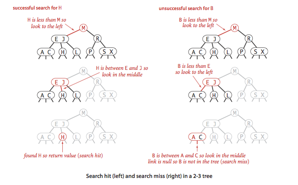
The search procedure for B-trees depends on the number of keys in a node.2
To determine whether a key is in a 2-3 tree, we compare it against the keys at the root: If it is equal to any of them, we have a search hit; otherwise, we follow the link from the root to the subtree corresponding to the interval of key values that could contain the search key, and then recursively search in that subtree.
Bruce Reed. 2003. The height of a random binary search tree. J. ACM 50, 3 (May 2003), 306–332. DOI: https://doi.org/10.1145/765568.765571 ↩
Robert Sedgewick and Kevin Wayne. Algorithms, Fourth Edition. 2011. Balanced Search Trees. https://algs4.cs.princeton.edu/33balanced/ ↩