Description

In computer graphics, we have long used the technique called “rasterization” to display a 3D scene as a 2D image. In the process, the triangles that represent the scene get projected on a plane, then the “shader” determines the color of each pixel within the triangle based on the triangle’s orientation, the light sources, and the material of the objects. In the first part of the project, you will learn how to implement a basic shader based on the Blinn-Phong Model.

Although rasterization can render a scene in real time, it could not handle translucent objects, refractions, and reflection to produce photorealistic images. In the second part of the project, you will be implementing another rendering technique called “ray tracing”, which can handle complex phenomena such as refraction, inter-reflections, caustics, and soft shadows. The only downside to this method is that it is significantly slower to compute.

Getting Started

Clone the GitLab repository that has been created for you. The skeleton code has comments marked with // TODO denoting where to write your code. You are encouraged to read through this document and review the Shading and Ray Tracing lectures carefully. The sample solution is only for the ray tracing part and only shows the debug rays.

The skeleton code is also avaliable here.

Overview

A shader is a program that controls how each point on the screen appears as a function of viewpoint, lighting, material properties, and other factors. Vertex shaders are run once for each vertex in your model. They transform it into device space (by applying the model view and projection matrices), and determine what each vertex’s properties are. Fragment (or pixel) shaders are run once for every pixel to determine its color. In this project, specifically, we will implement the Blinn-Phong shader. The equation is shown here:

$$I_\text{direct} = k_e + k_d I_a + \sum_j \Big[ A^\text{shadow}_j A^\text{dist}_j I_{L, j} \big( k_d (N \cdot L_j)_+ + k_s (N \cdot H_j)_+^{n_s} \big)\Big]$$

where $k_d$, $k_d$, $k_d$ are emissive, diffuse, and specular component of object; $n_s$ is the specular exponent (shininess); $I_a$ is the ambient light intensity; $I_L$ is the light intensity (product of intensity and color); $A^{\text{shadow}}$ and $A^{\text{dist}}$ are the shadow and distance attenuation; and $(\cdot)_+$ denotes $\max (0, \cdot)$.

Modern shaders and renderers support different types of light sources such as point light, directional light, and area light, but we will only focus on point light. Point light emits light from a single point in space, and its intensity is proportional to $1/r^2$ where $r$ is the distance from the light. In this implementation, we use set the distance attenuation to $1 / (1 + r^2)$ to avoid values greater than 1.

Implementation

There are 2 files that you need to look at:

• Assets/Shaders/BlinnPhong.shader: a file that defines a Shader object in Unity. You don’t have to edit this file, but it is important to look at the Properties since you will make use of these variables. The Transparency variables are not used in the Blinn-Phong specular reflection model and are only used in Ray Tracing below.
• Assets/Shaders/BlinnPhong.cginc a file that is included in the shader file above. Follow the // TODO in the function MyFragmentProgram to calculate the Blinn-Phong specular reflection model for point light.

Shader files are written in HLSL (High-level shader language) which is quite similar to C/C#. In the function MyFragmentProgram, we already implemented the emissive and diffuse component to demonstrate how we incorporate Unity’s built-in shader variables that you are probably going to use in your code.

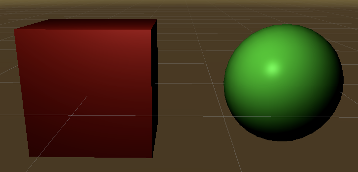
To see how the diffuse shader looks, go to the scene TestBlinnPhong, and observe how objects look under a point light. You will probably notice that there is a harsh falloff on the objects since the “attenuation” variable is not properly calculated.

Follow the TODOs to implement the required components. Specifically, you will need to calculate the distance attenuation for point light and calculate the ambient and specular components.

You are free to experiment with this scene. Here are some resources if you want to explore more about Unity’s shaders:

• Microsoft’s HLSL documentation for useful Vector functions used to calculate directional vectors such as vertex normal, camera view, etc.
• Built-in shader variables Lighting section to understand how Unity stores lighting data.
• Vertex data to learn more about how vertex data of objects is passed into shader functions.

Testing

It is recommended that you open the scene TestBlinnPhong where you can play around and add objects as you need. To create additional meshes and apply the Blinn-Phong shader, select the material → Shader → Custom → Lighting → BlinnPhong. You must not modify any other scenes except for TestBlinnPhong. Other scenes must be kept static for your benefit of matching the solution.

Whenever you edit the code in BlinnPhong.cginc, Unity will automatically update the scene from the Scene tab (left), meaning that you don’t have to press Play to see the result on the Game tab (right).

Overview

The ray tracer iterates through every pixel in the image, traces a ray from the camera through that point on the image plane, and calculates what color intensity to assign to that pixel based on the interaction of that ray (and recursively spanned rays) with the scene.

The skeleton code goes through several functions to do this, but most of the action occurs in the TraceRay() function. The function takes a ray as an input and determines the color that should be projected back to whatever that casts the ray. The function takes four arguments (two are used for debugging):

• ray: The ray to trace. A ray has an origin and a direction.
• recursionDepth: The current recursion depth (also see the variable MaxRecursionDepth)
• debug: (debugging purposes only) A boolean to control whether it should draw debug rays. You don’t need to modify this variable and just need to pass it along to the recursion tree.
• rayColor: (debugging purposes only) A color that represents the ray type in the debug visualization (reflection rays are blue, refraction rays are yellow, and shadow rays are magenta; these constants are already define at the top of the file)

First, the function determines if the ray actually intersects any objects in the scene. This is where a test for ray/object intersection occurs (see next section). If no intersection occurs, then a black color is returned (the zero vector). If an intersection occurs, the intersection data is saved into the variable hit. You will then use this variable to do shading calculations and possibly cast more rays, recursively.

The following diagram represents the flow of the ray tracing program:

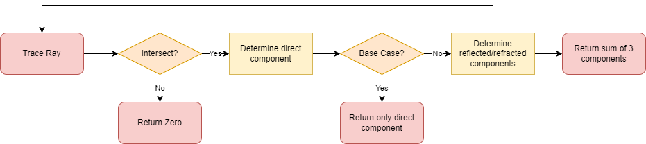
You will need to fill out the TODOs in the TraceRay() function.

Determining Color

There are three different components that contribute to the color of a surface:

• Direct Component
  • In the Blinn-Phong shading model, there are 4 subcomponents: emissive, ambient, diffuse, and specular. The equation is the same as in Part A.
  • The ambientColor is fetched from Unity’s lighting setting which can be accessed from Window → Rendering → Lighting → Environment → Environment Lighting.
  • You will need to iterate over every light source in the scene (see _pointLightObjects) and sum their individual contributions to the color intensity.
  • or each light, you will need to calculate the distance attenuation using $1/(1 + r^2)$ where $r$ is the distance from the intersection to the light source.
  • For calculating the shadow attenuation, implement the color-filtering through transparent objects as discussed in class. See Marschner Shirley Handout Section 4.7. You may create a separate function for shadow attenuation.
• Reflected Component
  • You will need to calculate the reflection vector, and then make a recursive call to the TraceRay() function.
  • See equations below on how to compute reflection ray. See also Marschner Shirley Handout Section 4.8.
• Refracted Component
  • Like the reflective component, this also needs to make recursive calls to the TraceRay() function. In addition, you also need to do some tests for total internal refraction and handle this case accordingly.
  • You can skip refraction if the object is opaque.
  • See equations below on how to compute refraction ray. See also Marschner Shirley Handout Section 13.1 (Ignore Fresnel term and Beer’s Law)
  • You may assume that objects are not nested inside other objects. If a refracted ray enters a solid object, it will pass completely through the object and back outside before refracting into another object.

Equations for Ray Tracing

$$I_\text{total} = I_\text{direct} + k_s I_\text{reflection} + k_t I_\text{refraction}$$

Reflection Direction

$$\mathbf{R} = 2 (\mathbf{V} \cdot \mathbf{N}) \mathbf{N} - \mathbf{V}$$

Refraction Direction

$$\eta = \eta_i / \eta_t$$

$$\cos \theta_i = \mathbf{N} \cdot \mathbf{V}$$

$$\cos \theta_t = \sqrt{1 - \eta^2(1 - \cos^2 \theta_i)}$$

$$\mathbf{T} = (\eta \cos \theta_i - \cos \theta_t)\mathbf{N} - \eta\mathbf{V}$$

Note that Total Internal Reflection (TIR) occurs when the square root term above is negative

Intersections

This section provides some explanation on how ray-object intersections are handled. You don’t need to implement anything here.

In TraceRay(), intersections are checked in the bvh.IntersectBoundingBox(Ray r, out Intersection hit) function which takes in a ray r and returns a boolean value of whether there is an intersection. The function also returns the intersection data through a pass by reference parameter hit for you to use. (Check bvh.cs in Assets\Scripts\Utilities if you want to know more)

The IntersectBoundingBox simply checks if a ray intersects with some bounding box. In our program, objects are divided and grouped into some bounding boxes based on their proximity. This is simply an acceleration structure which attempts to reduce the number of ray-object intersection checks as much as possible. The real ray-object intersection tests occur in the IntersectionLocal in the Utilities class where a ray is checked if it intersects with a sphere or a triangle face and returns the intersection data. The implementation details for ray-sphere and ray-triangle intersection check is from the Marschner Shirley Handout 4.4.1 and 4.4.2.

Testing Scenes

Go to the Tracer/Assets/Samples/ folder to see the solution’s rendered images.

Once you implement the requirements, you will be able to verify your implementation. Go to the Assets/Scenes/TestRayTracing folder and open the pre-made scenes and hit Play. After ray tracing a scene, the program will save a picture of the rendered scene into the Tracer/Assets/Students/. You will be notified by the text “Image Saved” on the screen.

Go to the Assets/Scenes/ImageComparison scene and click Play. The program will output a percentage for each scene. This percentage is how much your rendered scene matches the solution’s.

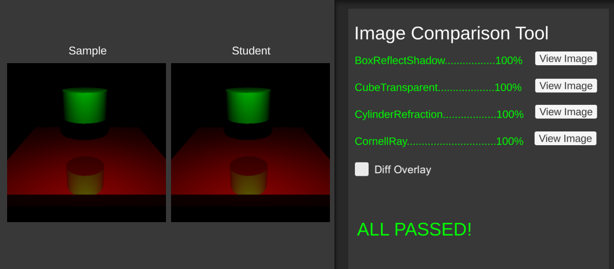
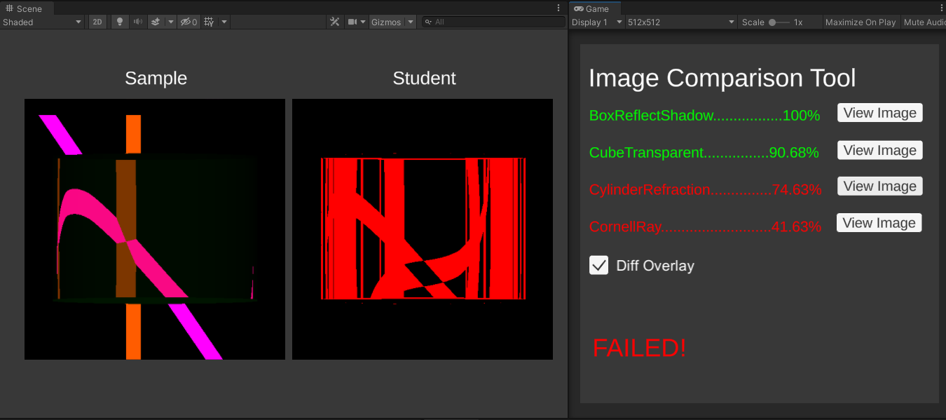
Turning on “Diff Overlay” shows the visual difference between the Sample image and the Student image. Any differences will be marked with red.

Here is what it looks like when “Diff Overlay” is off.

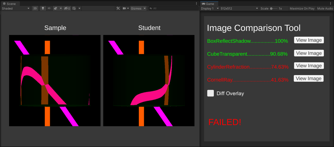
Check the Console for reasons that your scene may fail. Don’t worry if your solution doesn’t give exactly the same output (rounding errors, among other things, are a fact of life). Getting > 95% correct makes you pass a scene. However, if there is a noticeable pattern in the errors, then that definitely means something is wrong! This tool is only to get an idea of where to look for problems.

Ray Tracing Program Notes

You will probably spend the most of the time with the scripts in the Scripts/RayTracing folder, but you only need to edit the file RayTracer.cs. The Utilities folder, which you should not modify, contains the grade checker (ImageComparison.cs), acceleration structure for intersection calculations (BVH.cs), and some helpful imported libraries.

Important notices:

• Do not modify the sample scenes (except for TestBlinnPhong), as we will use these scenes to compare your result against the solution. If you need to ray trace a scene of your own, simply duplicate our scene (Ctrl/Command + D on any of our Scenes) and modify the copy.
• We recommend that you import our Unity layout for this project. From the top-right corner of the screen, select Layout → Load Layout From File and choose Assets/Layouts/TracerLayout.wlt. This makes Unity to show the Scene tab on the left, and the Game tab on the right for your convenience. Here is what the layout looks like:
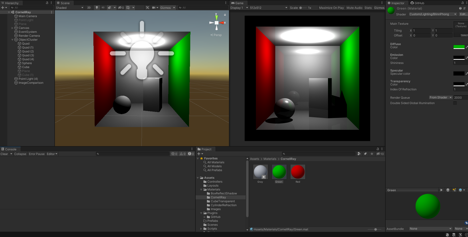  Notice that the Scene tab on the left has the barebone Unity objects which have Blinn-Phong shader as their material. The Game tab on the right is the ray-traced result. If you import our layout as recommended above, the 2 tabs will be automatically arranged like this to aid in the debugging process.
• All mesh objects (cube, sphere, cylinder, etc…) must have their material use the Blinn-Phong shader. To do so, create a new material, and set its shader to be Custom/Lighting/BlinnPhong. Refer to the materials from our sample scene to see how they are set up.

Custom Scene

You must also create a custom scene, separate from the sample scenes. In this scene, you should showcase any bells and whistles you have implemented. Make sure that any implemented bells and whistles do not affect the output of the sample scenes, as this will cause incorrect comparison results in the image comparison tool. This can be achieved in different ways, whether that be adding a flag in RayTracer.cs or in your material.

To create the scene, you may either start from scratch or modify a copy of one of the sample scenes. If you choose to modify one of the sample scenes, you must transform the scene in a resonably significant way (i.e. not only changing the camera angle). Doing this will lose points. This part of the project is where you get to showcase anything cool you created, so spend some time on it!

Debug Ray

Because out ray tracer can be hard to debug (“why is my image blank??”), we provide a visual debugging tool that helps you visualize which rays you’re tracing for each pixel. To use it, simply click Play for your scene, then click on a pixel of a rendered scene on the Game tab on the right, and check out how the ray traverses in space in the Scene tab on the left. Here is an example:

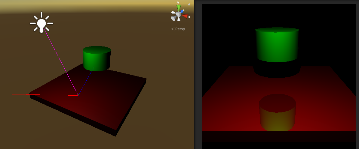
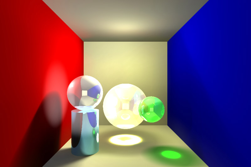
In this example, the user clicks on a reflection of the cylinder on the right pane (white mouse arrow), which results in these rays showing up in the left pane.

• Camera Ray (Red) The ray from our camera to the scene location is clicked on in the Game tab (right pane). This is the first ray that we will cast in order to trace the scene through that pixel.
• Shadow Ray (Magenta) The ray travels from the surface intersection points of the above rays to the light sources. A shadow ray either terminates at the light source, or intersects another surface along the way, indicating the presence of a shadow.
• Reflection Ray (Blue) The ray hits a surface and then bounces off based on the reflection model.
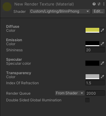
• Refraction Ray (Yellow) These rays are spawned through objects whose TransparentColor is non-zero. The ray’s direction is determined by the IndexOfRefraction in the object’s material.
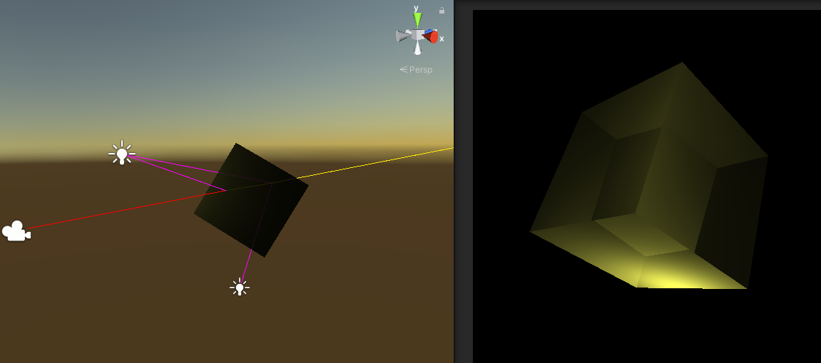  Here is an example material of the yellow cube above which makes it transparent:
  

Please follow the general instructions here.

Artifact Submission

For the artifact, turn in a screenshot of the custom raytraced scene you created. There is room here to create something really interesting, as ray traced scenes can have some really cool properties!

If you end up implementing a bell or whistle that can be animated, such as depth of field or motion blur, you may also include a video showcasing it. For example, you could animate the camera or other objects to showcase the scene. With complex ray tracers, this will most likely take a very long time to complete, but will look very cool, so make sure to get a nice looking static image first before doing this.

You are required to implement at least one bell and one whistle. You are also encouraged to come up with your own extensions for the project. Run your ideas by the TAs or Instructor, and we'll let you know if you'll be awarded extra credit for them. See syllabus for more information regarding extra credit and Bells and Whistles.

If you implement any bells or whistles you need to provide examples of these features in effect. You should present your extra credit features at grading time either by rendering scenes that demonstrate the features during the grading session or by showing images you rendered in advance. You might need to pre-render images if they take a while to compute (longer than 30 seconds). These pre-rendered examples, if needed, must be included in your turnin directory on the project due date. The scenes you use for demonstrating features can be different from what you end up submitting as an artifact.

Both Marschner and Shirley's book and Foley, et al., are reasonable resources for implementing bells and whistles. In addition, Glassner's book on ray tracing is a very comprehensive exposition of a whole bunch of ways ray tracing can be expanded or optimized (and it's really well written). If you're planning on implementing any of these bells and whistles, you are encouraged to read the relevant sections in these books as well.

Here are some examples of effects you can get with ray tracing. Currently, none of these were created from past students' ray tracers.

	Implement an adaptive termination criterion for tracing rays, based on ray contribution. Control the adaptation threshold with a slider or spinbox.
	Modify shadow attenuation to use Beer's Law, so that the thicker objects cast darker shadows than thinner ones with the same transparency constant. (See Marschner Shirley p. 325.)
	Include a Fresnel term so that the amount of reflected and refracted light at a transparent surface depend on the angle of incidence and index of refraction. (See Marschner Shirley p. 325.)
	Implement spotlights. You’ll have to extend the parser to handle spot lights but don’t worry, this is low-hanging fruit.
	Improve your refraction code to allow rays to refract correctly through objects that are contained inside other objects.
	Deal with overlapping objects intelligently. While the skeleton code handles materials with arbitrary indices of refraction, it assumes that objects don’t intersect one another. It breaks down when objects intersect or are wholly contained inside other objects. Add support to the refraction code for detecting this and handling it in a more realistic fashion. Note, however, that in the real world, objects can’t coexist in the same place at the same time. You will have to make assumptions as to how to choose the index of refraction in the overlapping space. Make those assumptions clear when demonstrating the results.
2x	Add a menu option that lets you specify a background images cube to replace the environment’s ambient color during the rendering. That is, any ray that goes off into infinity behind the scene should return a color from the loaded image on the appropriate face of the cube, instead of just black. The background should appear as the backplane of the rendered image with suitable reflections and refractions to it. This is also called environment mapping. Click here for some examples and implementation details and here for some free cube maps (also called skyboxes).
2x	Implement bump mapping. Check this and this out!
2x	Implement solid textures or some other form of procedural texture mapping. Solid textures are a way to easily generate a semi-random texture like wood grain or marble. Click here for a brief look at making realistic looking marble using Ken Perlin’s noise function.
2x *	Implement Monte Carlo path tracing to produce one or more or the following effects: depth of field, soft shadows, motion blur, or glossy reflection. For additional credit, you could implement stratified sampling (part of “distribution ray tracing”) to reduce noise in the renderings. (See lecture slides, Marschner Shirley 13.4). *You will earn 2 bells for the first effect, and 2 whistles for each additional effect.
2x *	Implement caustics by tracing rays from the light source and depositing energy in texture maps (a.k.a., illumination maps, in this case). Caustics are variations in light intensity caused by refractive focusing–everything from simple magnifying-glass points to the shifting patterns on the bottom of a swimming pool. Here is a paper discussing some methods. 2 bells each for refractive and reflective caustics. (Note: caustics can be modeled without illumination maps by doing “photon mapping”, a monster bell described below.) Here is a really good example of caustics that were produced by two students during a previous quarter: Example

Sub-Surface Scattering The trace program assigns colors to pixels by simulating a ray of light that travels, hits a surface, and then leaves the surface at the same position. This is good when it comes to modeling a material that is metallic or mirror-like, but fails for translucent materials, or materials where light is scattered beneath the surface (such as skin, milk, plants... ). Check this paper out to learn more.

Photon Mapping Photon mapping is a powerful variation of ray tracing that adds speed, accuracy and versatility. It's a two-pass method: in the first pass photon maps are created by emitting packets of energy photons from the light sources and storing these as they hit surfaces within the scene. The scene is then rendered using a distribution ray tracing algorithm optimized by using the information in the photon maps. It produces some amazing pictures. Here's some information on it. Also, if you want to implement photon mapping, we suggest you look at the SIGGRAPH 2004 course 20 notes (accessible from any UW machine or off-campus through the UW library proxy server).