Shortest Paths Reading
Complete the Reading Quiz by 3:00pm before lecture.
In the previous lecture, we learned about how different graph implementations resulted in different runtimes for depth-first search and breadth-first search.
- DFS
- Find a path from a given vertex, s, to every reachable vertex in the graph.
- BFS
- Find a shortest path from a given vertex, s, to every reachable vertex in the unweighted graph.
- Dijkstra’s Algorithm
- Find a shortest path from a given vertex, s, to every reachable vertex in a weighted graph.
Remember that we arrived at Dijkstra’s algorithm in lecture by swapping out the Queue used in BFS for a PriorityQueue, ensuring that the lowest-weighted edges are explored first at each point in the algorithm. The following pseudocode walks through Dijkstra’s algorithm:
dijkstras(Node s, Graph g) {
    PriorityQueue unvisited;
    unvisited.addAll(g.allVertices(), ∞);
    unvisited.changePriority(s, 0);

    Map<Node, Integer> distances;

    while (!unvisited.isEmpty()) {
        Node n = unvisited.removeMin();
        for (Node i : n.neighbors) {
            if (distances[i] < distances[n] + g.edgeWeight(n, i)) {
                continue;
            } else {
                distances[i] = distances[n] + g.edgeWeight(n, i);
                unvisited.changePriority(i, distances[i]);
            }
        }
    }
}
The visualization below shows an example of Dijkstra’s algorithm in action:
Make sure you understand how Dijkstra’s works before proceeding. Although the algorithm is useful in an incredible number of applications within computer science, it isn’t always the best choice: the next two sections each cover a limitation.
Limitation: Negative Edge Weights
We mentioned in lecture that Dijkstra’s can fail on graphs with negative edge weights. Let’s look at a small example where this is the case.
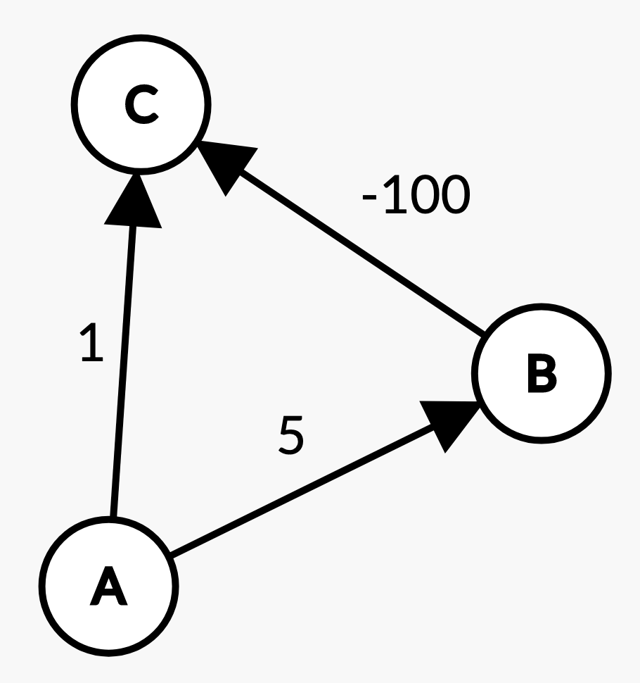
What path does Dijkstra's select from vertex A to vertex C?
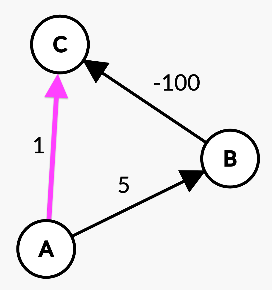
Dijkstra’s chooses its paths greedily; when visiting A, Dijkstra’s thought the shortest path to C utilized the edge with path weight 1. However, by visually inspecting the graph that the actual shortest path between A and C is through B for a total path weight of -95. This is because when Dijkstra’s finally visited B and discovered the edge with -100, it didn’t update C’s shortest path; Dijkstra’s will not update nodes which are not in the fringe.
Also remember that Dijkstra’s (and any other shortest path algorithm) is guaranteed to fail on any graph that contains a cycle whose overall weight is negative (ie, negative weight cycle). In fact, the “shortest path” isn’t defined on a graph with a negative weight cycle. The more times you traverse the negative weight cycle, the lower your path weight becomes, and since it’s a cycle, this can be done infinitely many times, effectively achieving an infinitely small path weight.
Limitation: Searching Many Nodes
Even with all positive edges, there are some situations where Dijkstra’s isn’t the best choice. Suppose we have a graph laid out in a grid, as below, and we want to find path from s to t.
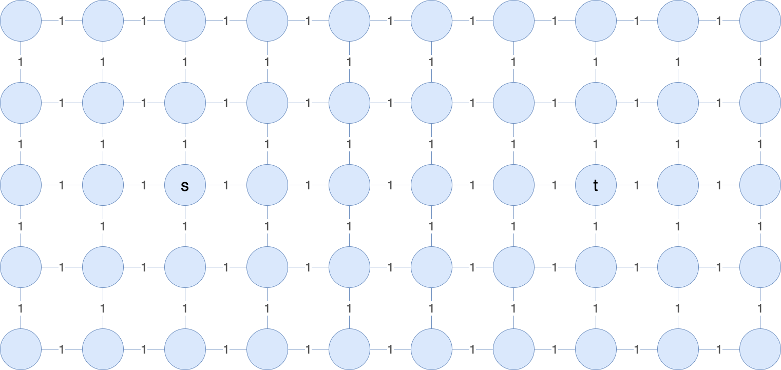
How will Dijkstra’s algorithm run on the graph? It will find the correct path from s to t by searching edges starting from s in all directions until it eventually finds t. Just like BFS, Dijkstra’s traverses all the nodes it can, so many nodes in the graph will be covered before finding t. We can see visually that the node immediately to the left of s will not be on s’s shortest path to t, but BFS and Dijkstra’s will still search it.
Could we improve on this behavior? Notice that in this simple grid graph, it is generally preferable for our shortest path search to travel to the right from node s when finding a path to t. It’s easy to see why visually, but that fact isn’t encoded anywhere in the graph’s edge weights. For our shortest path algorithm to take advantage of that extra information, we need a way for it to determine a “preference” among the available nodes it could visit.
We’d like to give the algorithm info about how far each node is from t, so it can tend toward picking the closest ones. Unfortunately, computing that distance is the same problem we’re trying to solve, so we’d need to run an entirely new instance of Dijkstra’s to solve it completely. Luckily, we have prior knowledge about this particular graph: that it is laid out in a grid with edge weights of 1. Using that knowledge, it’s efficient to approximate the distance.
Approximating Distances via Heuristics
We could calculate the “physical” (sometimes known as Euclidean) distance from each node to t fairly easily: take the square root of the summed-squared vertical and horizontal offsets in the grid. But an even easier approximation is simply adding up the vertical and horizontal offsets; this is known as the Manhattan distance.
What would the computed Manhattan distances look like for this graph?
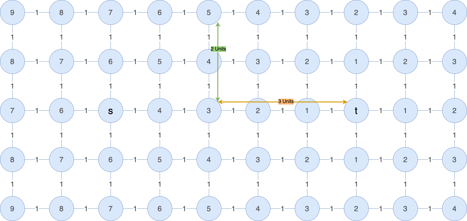
Note how the highlighted node has a Manhattan distance of 5 because it is 2 units above and 3 units to the left of t.
Computing the Manhattan distance is an example of a heuristic: a strategy for comparing nodes in the graph, based on properties of the problem. Even though it is just an approximation, the Manhattan distance computation is a useful heuristic because it:
- decreases as we get “closer” to the goal
t(for some definition of distance) - is efficient to compute
The heuristic estimates graph-distance (ie, distance of the shortest path) using some other form of distance that we have prior knowledge of (ie, Manhattan distance). Importantly, the reason it’s even possible to talk about the Manhattan/Euclidean distance between nodes in this graph is because it’s laid out in a grid, so there is a meaningful notion of which nodes are close to each other “in space”.
At a high level, how would you make a modified version of Dijkstra's algorithm to take advantage of the prior knowledge for the grid graph?
Rather than sorting nodes in the Priority Queue based solely on their edge weights, we could also incorporate information about their distance to t. That way, given the choice between two nodes reachable by similar edge weights, we could prioritize visiting the one that we know lies closer to t.
For a more graphical explanation of the difference between Dijkstra’s algorithm (which doesn’t use this kind of heuristic) vs. a hypothetical shortest path algorithm with heuristic data, say we want to find path between two points in a geographical map:
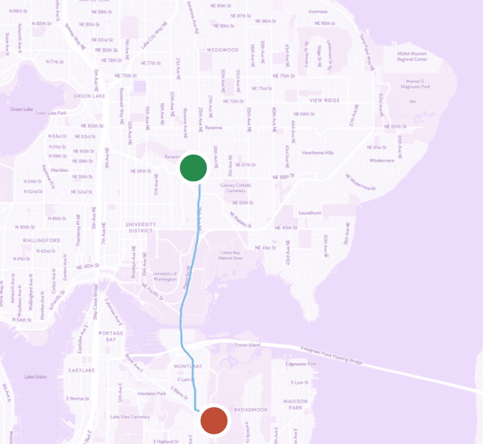
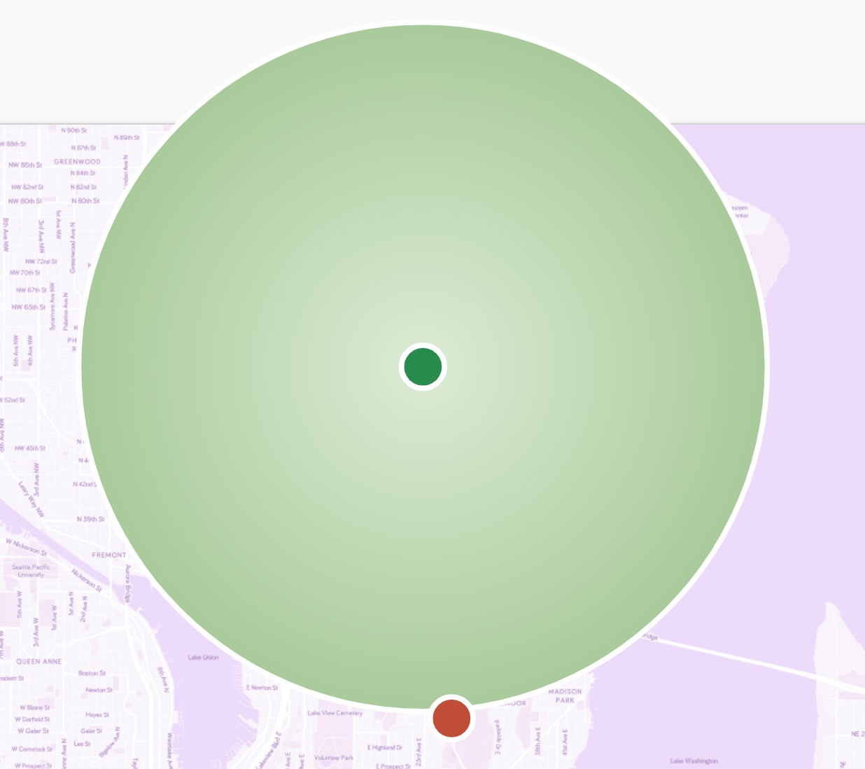
The points searched by Dijkstra’s will resemble a circle, as it explores in all directions:
But if we had access to prior knowledge about the relative direction of points on the map, we could “focus” our exploration:
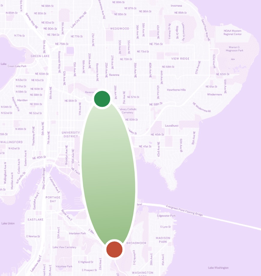
In lecture, we will examine the latter type of algorithm: one that can take advantage of that information.