Seam Carving
Implement a content-aware image resizing algorithm.1
Learning goals
Solve a real-world graph problem via reduction.
Reduction is an important tool in computer science theory, but it also has practical applications for solving real-world problems. One of the building blocks of computer science is the idea of abstraction, and reductions represent one of the strongest forms of abstractions by using the solution to one problem as a “black box” for solving a different but somehow related problem.
Represent problem solutions as states in a graph.
In class, we presented several graph algorithms for solving a variety of classical graph problems including shortest paths and minimum spanning trees. But in the real-world, problems rarely immediately jump out as solvable with graph algorithms. How we represent the problem as a graph is one of the most important decisions as it determines which algorithms we can employ to solve the problem.
Apply graph augmentation as a strategy for solving a new class of graph problems.
After coming up with a graph representation of the problem (an abstraction), we can then formally define the problem in terms of the abstraction. However, our problem still might be hard to solve! In seam carving, we need to find the weighted shortest path from any vertex in a distinguished set S to another set T. One common strategy for solving these problems is by augmenting the graph with additional nodes or edges.
Table of contents
Due Date
Please be forewarned that we will not accept late submissions beyond the 9pm due date because of the grade submission deadline.
Overview
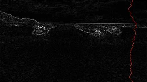
Seam-carving is a content-aware image resizing technique where the image is reduced in size by one pixel of height (or width) at a time. A vertical seam in an image is a path of pixels connected from the top to the bottom with one pixel in each row; a horizontal seam is a path of pixels connected from the left to the right with one pixel in each column. Below left is the original 505-by-287 pixel image; below right is the result after removing 150 vertical seams, resulting in a 30% narrower image. Unlike standard content-agnostic resizing techniques (such as cropping and scaling), seam carving preserves the most interest features (aspect ratio, set of objects present, etc.) of the image.
Although the underlying algorithm is simple and elegant, it was not discovered until 2007. Now, it is now a core feature in Adobe Photoshop and other computer graphics applications.


In this assignment, you will create a data type that resizes a -by- image using the seam-carving technique. Finding and removing a seam involves three parts and a tiny bit of notation.
Getting the Assignment
- Task
- Pull the
skeletonrepository to get theseamcarvingassignment.
If IntelliJ doesn’t properly recognize the new files or complains about failing to resolve classes or interfaces from previous assignments, refresh Gradle manually through the Gradle tool window (on the right by default):

Seam Carving Algorithm
- Background
- Read through the description of the seam carving algorithm.
Notation: In image processing, pixel refers to the pixel in column and row , with pixel at the upper-left corner and pixel at the lower-right corner. This is consistent with the Picture data type that we use in this assignment.
A 3-by-4 image.
- Warning
- This is the opposite of the standard mathematical notation used in linear algebra, where refers to row and column and is at the lower-left corner.
We also assume that the color of each pixel is represented in RGB space, using three integers between 0 and 255. This is consistent with the Color data type.
Energy calculation. The first step is to calculate the energy of a pixel, which is a measure of its importance—the higher the energy, the less likely that the pixel will be included as part of a seam (as you will see in the next step). In this assignment, you will use the dual-gradient energy function, which is described below. Here is the dual-gradient energy function of the surfing image above:
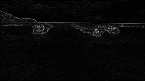
The energy is high (white) for pixels in the image where there is a rapid color gradient (such as the boundary between the sea and sky and the boundary between the surfing Josh Hug on the left and the ocean behind him). The seam-carving technique avoids removing such high-energy pixels.
Seam finding. The next step is to identify a vertical seam of minimum total energy. (Finding a horizontal seam is analogous.) This is similar to the classic shortest path problem in an edge-weighted digraph, but there are three important differences:
- Each edge weight is based on a vertex (pixel) rather than the edge itself.
- The goal is to find the shortest path from any of the pixels in the top row to any of the pixels in the bottom row.
- The digraph is acyclic, where there is a downward edge from pixel to pixels , , and , assuming that the coordinates are in the prescribed ranges.
Seams cannot wrap around the image (e.g., a vertical seam cannot cross from the leftmost column of the image to the rightmost column).
Seam removal. The final step is remove from the image all of the pixels along the vertical or horizontal seam. This has already been implemented for you in the
SeamCarverclass.
Dual-Gradient Energy Function
- Task
- Implement
DualGradientEnergyFunctionusing the following math.
For this assignment, we are going to define the energy of a pixel to be the magnititude of the rate of change of colors at that pixel. In other words, a high energy pixel is one that has a large change from its neighbors while a low energy pixel has very little change between itself and its neighbors. The way we are actually going to calculate this value is by approximating the derivative in the X and Y directions then combine these using the pythagorean theorem to get the overall change.
To start, we need to figure out how to calculate the derivative which in more than one dimension is called the gradient. Usually, when we find derivatives we have a continuous function to look at, but here we only have the descrete pixels making up our picture. This means we will have to use something called numerical differentiation that (luckily) some very smart mathematicians have already figured out for us. For our assignment, we will be using two formulas to calculate the gradient. The first is called the Central Difference and is defined as follows:
Where and represent the gradient of in the direction and direction respectively. These functions are very useful if we know the values of surrounding a point , but if we do not know or cannot calculate we cannot use these functions. This means our approximation method won’t work on the edges of our picture where we don’t have pixels on all sides. Instead, we use a second approximation called the Forward/Backward Difference which is defined as:
Where can be either 1 or -1. When it is 1 we call it the Forward Difference because the points are increasing and when it is -1 we call it the Backward Difference since the points are decreasing. As you can see, this allows us to calculate the approximate value of and on the edges of the picture since our formula only involves points on one side of x and y. One note for pedantics is that the true value of the gradient is actually scaled and may have a different sign from what we are calculating, but since we will eventually be squaring these numbers and only care about the relative values, this ends up not impacting our calculations.
Now, we need to use these approximations to calculate the overall energy at a pixel. First, we will use , , and to represent the red, green, and blue values of the pixel located at . Each one of these function also has an and gradient like our function above which we will denote using the same subscripts of and . We can now define the square of the total rates of change in the and direction to be:
Where and the related functions can be approximated using the method above. Then, for the final part, we need to use the Pythagorean theorem to combine these two values to get the magnitude of the change which gives us our final formula for energy:
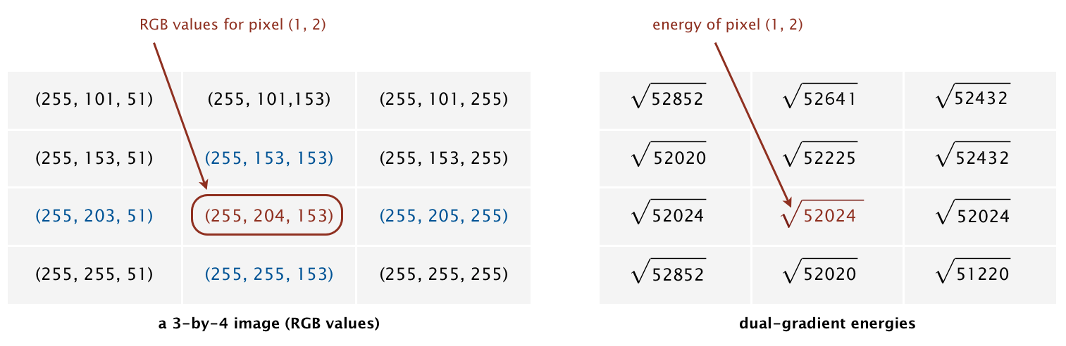
As an example, consider the 3-by-4 image with RGB values (each component is an integer between 0 and 255) as shown in the table below. (This is the 3x4.png image in your seamcarving/data/ folder.)
Example 1
The energy of the non-border pixel is calculated using the central difference from pixels and for the x-gradient
yielding ;
and pixels and for the y-gradient
yielding .
Thus, the energy of pixel is .
What is the energy of pixel (1, 1)?
The energy of pixel is .
Example 2
The energy of the border pixel is calculated by the forward difference using pixels , , and for the x-gradient since it is on the left edge of the image
yielding .
Similarly, for the y-gradient we will use the backward difference using pixels , , and since the point is on the bottom edge of the image.
yielding .
Thus, the energy of pixel is .
Summary
The energy for each pixel is given in the table below.
| √52852 | √52641 | √52432 |
| √52020 | √52225 | √52432 |
| √52024 | √52024 | √52024 |
| √52852 | √52020 | √51220 |
Finding a Vertical Seam
- Task
- Implement
SeamFinder.findVerticalSeamby reducing the problem to one solvable using Dijkstra’s algorithm.
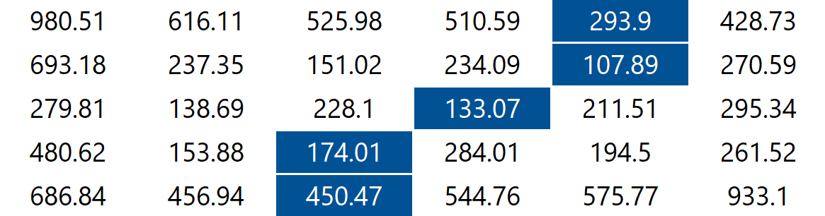
The findVerticalSeam method returns an array of length such that entry is the column number of the pixel to be removed from row of the image. Consider the 6-by-5 image (6x5.png) with RGB values shown in the table below.
| (78, 209, 79) | (63, 118, 247) | (92, 175, 95) | (243, 73, 183) | (210, 109, 104) | (252, 101, 119) |
| (224, 191, 182) | (108, 89, 82) | (80, 196, 230) | (112, 156, 180) | (176, 178, 120) | (142, 151, 142) |
| (117, 189, 149) | (171, 231, 153) | (149, 164, 168) | (107, 119, 71) | (120, 105, 138) | (163, 174, 196) |
| (163, 222, 132) | (187, 117, 183) | (92, 145, 69) | (158, 143, 79) | (220, 75, 222) | (189, 73, 214) |
| (211, 120, 173) | (188, 218, 244) | (214, 103, 68) | (163, 166, 246) | (79, 125, 246) | (211, 201, 98) |
The minimum energy vertical seam is highlighted in blue. In this case, the method findVerticalSeam returns the array [4, 4, 3, 2, 2] because the pixels in the minimum energy vertical seam are .
When there are multiple vertical seams with minimal total energy, your method can return any such seam.
Finding a Horizontal Seam
- Task
- Implement
SeamFinder.findHorizontalSeam, which should look very similar toSeamFinder.findVerticalSeam.
The behavior of findHorizontalSeam is analogous to that of findVerticalSeam except that it should return an array of length such that entry is the row number of the pixel to be removed from column of the image. For the 6-by-5 image, the method findHorizontalSeam returns the array [2, 2, 1, 2, 1, 1] because the pixels in the minimum energy horizontal seam are .
Runtime Requirements
- Task
- Meet the following runtime requirements:
- The runtime of
energyshould be in because it is a closed-form expression. - The runtime for finding either the vertical seam or the horizontal seam should both be in .
Tips
- Recommended
- Read these.
We’re reducing the seam carving problem to a shortest path problem that we can solve using Dijkstra’s algorithm; this has a number of implications:
- General reduction notes
- Before using
AStarPathFinder, we need to preprocess the problem into a formatAStarPathFindercan use. - After using
AStarPathFinder, we need to postprocess its output into the format theSeamFinderinterface needs.
- Before using
- Preprocessing for
AStarPathFinder- The path finder needs a graph to run on, so you’ll need to implement an
AStarGraphfor this reduction.- Here’s a rough specification for finding vertical seams:
- Vertices represent pixels.
- Edges exist from a pixel to its 3 downward neighbors.
- Edges have weight representing energy.
- The shortest (least total weight) path from top to bottom represents the minimum-energy seam.
- It might also be useful to look at the example graph implementations from the A* assignment. Notice that the graphs for puzzles don’t actually store a complete representation of the graph, instead opting to lazily generate the output for
neighborswhen the method gets called—this reduces the overall memory usage and runtime for large graphs which might otherwise cause Java to run out of memory.
- Here’s a rough specification for finding vertical seams:
- [!] The path finder needs a single vertex to start on, and a single vertex to end on. In the seam carving problem, there are multiple possible first and last pixels to choose, so we’ll need to do something else in the graph to allow the path finder to choose any valid seam. This is an important but unintuitive observation for this assignment!
- The path finder needs a graph to run on, so you’ll need to implement an
Testing
- Recommended
- Read these notes about the testing and grading.
We have not provided many unit tests with this assignment. Instead, we’ve included multiple images of various sizes in the seamcarving/data/ folder, along with the expected energies and seams indicated in text files. Feel free to run the provided demo applications and manually check your results against the expected ones in the text files, or practice writing unit tests by converting the expected results in the text files into equivalent tests.
Additionally, like the previous assignment, this assignment includes a method that creates a ShortestPathFinder, which we will override on the grader to use the solution implementation. We recommend using this so that you don’t get penalized again for any bugs or inefficiencies left over in your previous assignments.
Submission
Commit and push your changes to GitLab before submitting your homework to Gradescope.
🥳 Congratulations on completing all the assignments!
Josh Hug. 2015. Seam Carving. In Nifty Assignments 2015. http://nifty.stanford.edu/2015/hug-seam-carving/
Josh Hug, Kevin Wayne, and Maia Ginsburg. 2019. Seam Carving. In COS 226, Spring 2019. https://www.cs.princeton.edu/courses/archive/spring19/cos226/assignments/seam/specification.php ↩