Introduction and Energy Calculation

Determining the importance of pixels in an image.

Table of contents

1. Seam Carving Algorithm
   1. Notation
   2. Overview
2. Dual-Gradient Energy Function
   1. Runtime Requirements

Seam Carving Algorithm

Background

Read through the description of the seam carving algorithm.

Seam-carving is a content-aware image resizing technique where the image is reduced in size by one pixel of height (or width) at a time. A vertical seam in an image is a path of adjacent or diagonally-adjacent pixels connected from the top of the image to the bottom, with one pixel in each row; a horizontal seam is the same from left to right. (Seams cannot wrap around the image: e.g., a vertical seam cannot cross from the leftmost column of the image to the rightmost column.) Below left is the original 505-by-287 pixel image; below right is the result after removing 150 vertical seams, resulting in a 30% narrower image. Unlike standard content-agnostic resizing techniques (such as cropping and scaling), seam carving preserves the most interest features (aspect ratio, set of objects present, etc.) of the image.

Although the underlying algorithm is simple and elegant, it was not discovered until 2007. Now, it is now a core feature in Adobe Photoshop and other computer graphics applications.

In this assignment, you will create implement an algorithm that resizes a $W$-by-$H$ image using the seam-carving technique.

Notation

In image processing, pixel $(x, y)$ refers to the pixel in column $x$ and row $y$, with pixel $(0, 0)$ at the upper-left corner and pixel $(W - 1, H - 1)$ at the lower-right corner. This is consistent with the Picture data type that we use in this assignment.

A 3-by-4 image.

Warning

This is the opposite of the standard mathematical notation used in linear algebra, where $(i, j)$ refers to row $i$ and column $j$ and $(0, 0)$ is at the lower-left corner.

We also assume that the color of each pixel is represented in RGB space, using three integers between 0 and 255. This is consistent with the Color data type.

Overview

Finding and removing a seam involves three parts:

1. Pre-processing: The first step is to pre-process the image to determine the importance of each pixel. For each pixel, we calculate an energy, a measure of its distinctness from its adjacent pixels; the higher the energy, the more important it is. In this assignment, you will use the dual-gradient energy function, which is described below. Here are the values of the dual-gradient energy function on the surfing image above:

   

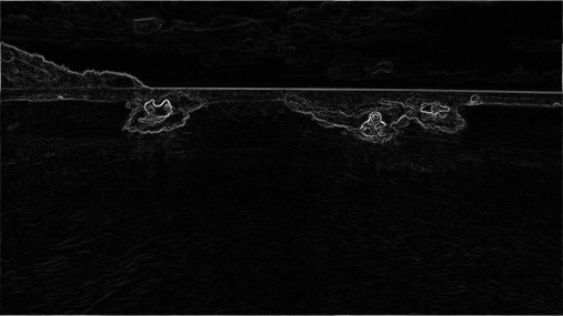
   The energy is high (white) for pixels in the image where there is a rapid color gradient (such as the boundary between the sea and sky and the boundary between the surfing Josh Hug on the left and the ocean behind him). The seam-carving technique will avoid removing such high-energy pixels.

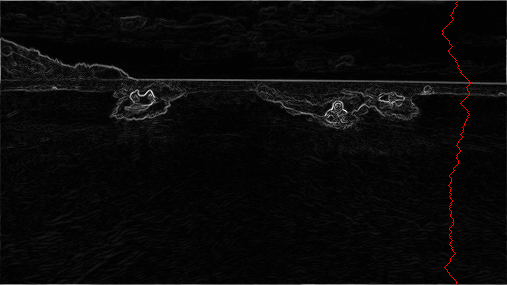
2. Seam finding: The next step is to identify a seam of minimum total energy. The direction of the seam depends on the dimension being resized: resizing horizontally requires vertical seams, and resizing vertically requires horizontal seams. Seam finding is similar to the classic shortest path problem in a weighted directed graph, but with some key differences that will be discussed later.

   

3. Seam removal: The final step is remove from the image all of the pixels along the vertical or horizontal seam. This has already been implemented for you in the SeamCarver class.

Dual-Gradient Energy Function

Task

Implement DualGradientEnergyFunction using the following math.

For this assignment, we are going to define the energy of a pixel to be the magnitude of the rate of change of colors at that pixel. In other words, a high energy pixel is one that has a large change from its neighbors while a low energy pixel has very little change between itself and its neighbors. The way we are actually going to calculate this value is by approximating the derivative in the X and Y directions then combine these using the pythagorean theorem to get the overall change.

To start, we need to figure out how to calculate the derivative which in more than one dimension is called the gradient. Usually, when we find derivatives we have a continuous function to look at, but here we only have the descrete pixels making up our picture. This means we will have to use something called numerical differentiation that (luckily) some very smart mathematicians have already figured out for us. For our assignment, we will be using two formulas to calculate the gradient. The first is called the Central Difference and is defined as follows:

$f_x(x, y) \approx f(x + 1, y) - f(x - 1, y)$
$f_y(x, y) \approx f(x, y + 1) - f(x, y -1)$

Where $f_x$ and $f_y$ represent the gradient of $f$ in the $x$ direction and $y$ direction respectively. These functions are very useful if we know the values of $f$ surrounding a point $(x, y)$, but if we do not know or cannot calculate $f(x - 1, y)$ we cannot use these functions. This means our approximation method won’t work on the edges of our picture where we don’t have pixels on all sides. Instead, we use a second approximation called the Forward/Backward Difference which is defined as:

$f_x(x, y) \approx -3 f(x, y) + 4 f(x + \delta, y) - f(x + 2 \delta, y)$
$f_y(x, y) \approx -3 f(x, y) + 4 f(x, y + \delta) - f(x, y + 2 \delta)$

Where $\delta$ can be either 1 or -1. When it is 1 we call it the Forward Difference because the points are increasing and when it is -1 we call it the Backward Difference since the points are decreasing. As you can see, this allows us to calculate the approximate value of $f_x$ and $f_y$ on the edges of the picture since our formula only involves points on one side of x and y. One note for pedantics is that the true value of the gradient is actually scaled and may have a different sign from what we are calculating, but since we will eventually be squaring these numbers and only care about the relative values, this ends up not impacting our calculations.

Now, we need to use these approximations to calculate the overall energy at a pixel. First, we will use $R(x,y)$, $G(x,y)$, and $B(x,y)$ to represent the red, green, and blue values of the pixel located at $(x,y)$. Each one of these function also has an $x$ and $y$ gradient like our function $f$ above which we will denote using the same subscripts of $x$ and $y$. We can now define the square of the total rates of change in the $x$ and $y$ direction to be:

$\Delta_x^2(x, y) = R_x(x, y)^2 + G_x(x, y)^2 + B_x(x, y)^2$
$\Delta_y^2(x, y) = R_y(x, y)^2 + G_y(x, y)^2 + B_y(x, y)^2$

Where $R_x$ and the related functions can be approximated using the method above. Then, for the final part, we need to use the Pythagorean theorem to combine these two values to get the magnitude of the change which gives us our final formula for energy:

$\operatorname{energy}(x, y) = \sqrt{\Delta_x^2(x, y) + \Delta_y^2(x, y)}$

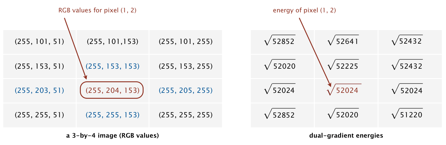
As an example, consider the 3-by-4 image with RGB values (each component is an integer between 0 and 255) as shown in the table below. (This is the 3x4.png image in your seamcarving/data/ folder.)

Example 1

The energy of the non-border pixel $(1, 2)$ is calculated using the central difference from pixels $(0, 2)$ and $(2, 2)$ for the x-gradient

$R_x(1, 2) = 255 - 255 = 0$
$G_x(1, 2) = 205 - 203 = 2$
$B_x(1, 2) = 255 - 51 = 204$

yielding $\Delta_x^2(1, 2) = 2^2 + 204^2 = 41620$;

and pixels $(1, 1)$ and $(1, 3)$ for the y-gradient

$R_y(1, 2) = 255 - 255 = 0$
$G_y(1, 2) = 255 - 153 = 102$
$B_y(1, 2) = 153 - 153 = 0$

yielding $\Delta_y^2(1, 2) = 102^2 = 10404$.

Thus, the energy of pixel $(1, 2)$ is $\sqrt{41620 + 10404} = \sqrt{52024}$.

Example 2

The energy of the border pixel $(0, 3)$ is calculated by the forward difference using pixels $(0, 3)$, $(1, 3)$, and $(2, 3)$ for the x-gradient since it is on the left edge of the image

$R_x(0, 3) = -3 \cdot 255 + 4 \cdot 255 - 255 = 0$
$G_x(0, 3) = -3 \cdot 255 + 4 \cdot 255 - 255 = 0$
$B_x(0, 3) = -3 \cdot 51 + 4 \cdot 153 - 255 = 204$

yielding $\Delta_x^2(0, 3) = 204^2 = 41616$.

Similarly, for the y-gradient we will use the backward difference using pixels $(0, 3)$, $(0, 2)$, and $(0, 1)$ since the point is on the bottom edge of the image.

$R_y(0, 3) = -3 \cdot 255 + 4 \cdot 255 - 255 = 0$
$G_y(0, 3) = -3 \cdot 255 + 4 \cdot 203 - 153 = -106$
$B_y(0, 3) = -3 \cdot 51 + 4 \cdot 51 - 51 = 0$

yielding $\Delta_y^2(0, 3) = (-106)^2 = 11236$.

Thus, the energy of pixel $(0, 3)$ is $\sqrt{41616 + 11236} = \sqrt{52852}$.

Summary

The energy for each pixel is given in the table below.

Runtime Requirements

Task

Make sure that the runtime of apply is in $\Theta(1)$.

After you have the energy function working, you can move on to implementing seam finding.