Reductions and Topological Sorting Reading
Reduction and Decomposition
In academia, data structures and algorithms courses like 373 are considered foundational computer science courses; in industry, they’re considered source material for standard interview questions. Why do academics and companies seek candidates with this specific knowledge?
One reason is that many problems – both theoretical and real-world – can be formulated in such a way that they’re solvable with the data structures and algorithms we’ve learned. This process of turning a real-world problem to a computable, abstract representation is called problem decomposition.
A special type of problem decomposition are reductions, which transform one problem into another problem. Reductions do not modify the algorithm itself. Instead, reductions follow a three-step process.
- Transform the input so that it can be solved by the standard algorithm.
- Run the standard algorithm as-is on the transformed input.
- Transform the output of the algorithm to solve the original problem.
Consider two methods for finding duplicates in a sorted array: one that compares every pair of items and another that uses the fact that the input is sorted to speed up running time. Here’s some code demonstrating the second, faster method.
public static boolean singlePassContainsDuplicate(int[] A) {
  for (int i = 0; i < A.length - 1; i += 1) {
    if (A[i] == A[i + 1]) {
      return true;
    }
  }
  return false;
}
Suppose we know that we can sort an array in θ(Nlog(N)) runtime. In such a case, finding a duplicate in an unsorted array reduces to sorting!
Duplicates: Are there any duplicate items in an array of Comparable objects? How many distinct items are there in an array? With sorting, you can answer these questions in θ(Nlog(N)) time: first sort the array, then make a pass through the sorted array, taking note of duplicate values that appear consecutively in the ordered array (as demonstrated in the code above).
What are the three reduction steps for reducing duplicate finding to sorting?
- No transformation to the input array.
- Sort the input array. (standard algorithm as-is)
- Scan over the sorted array. If there are adjacent duplicate items, return true. Otherwise, return false.
The example above demonstrates that not all reductions use all three steps. This reduction demonstrates, from a theoretical perspective, that finding duplicate items in an unsorted array is no more difficult than sorting (because the scanning step is both simpler and faster than the sorting itself).
Topological Sorts
Definition: Topological Ordering
Given a weighted directed acyclic graph (a DAG), put the vertices in order such that all its directed edges point from a vertex earlier in the order to a vertex later in the order (or report that doing so is not possible). This ordering is called a topological ordering.
Consider the following DAG:
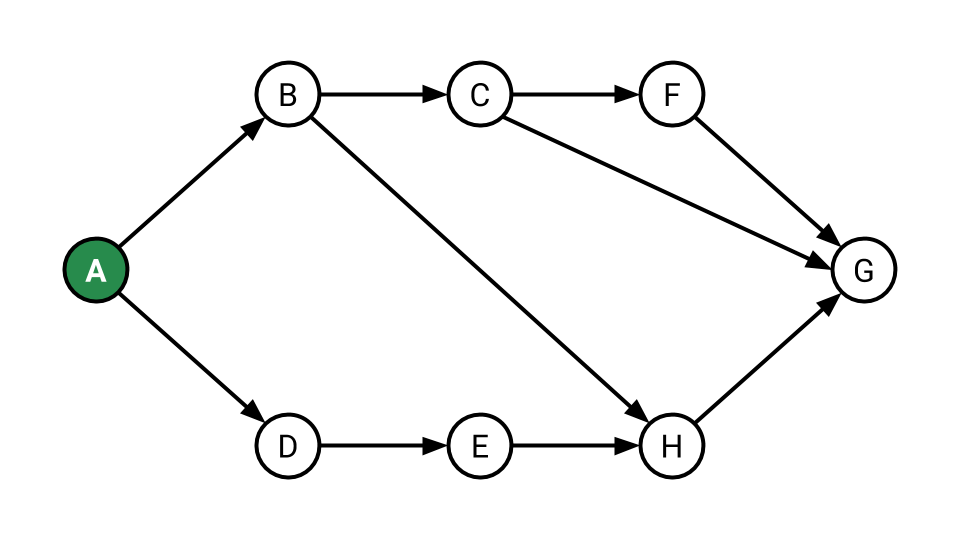
Give a topological ordering for the vertices in the graph.
A, B, D, E, H, C, F, G is one example. 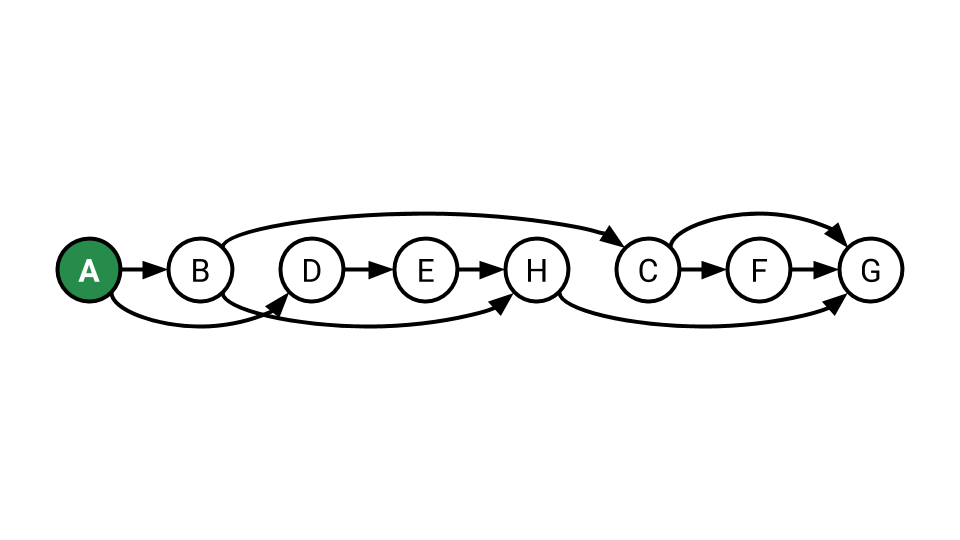
A, D, E, B, H, C, F, G is another. We can describe some of the constraints corresponding to each incoming edge.
The first vertex needs to be A.
- E must come after D.
- H must come after B and E.
- C must come after B.
- F must come after C.
- The final vertex needs to be G.
Algorithms to Calculate A Topological Ordering
What algorithm could we use to calculate this topological ordering? We can try a few flavors of depth-first search.
Give the DFS preorder traversal of the graph assuming we explore neighbors in alphabetical order.
A, B, C, F, G, H, D, E. This doesn’t satisfy the ordering constraints, so preorder traversals don’t work.
Give the DFS postorder traversal of the graph assuming we explore neighbors in alphabetical order.
G, F, C, H, B, E, D, A. The result is backwards: all of the constraints are in reverse.
A valid topological ordering can be computed by reversing the DFS postorder traversal starting from a vertex with no incoming edges. In case not every vertex is reachable from the starting vertex, it’s necessary to “restart” the reverse DFS postorder traversal from another vertex with no incoming edges.
Adapting Dijkstra’s for negative-weighted DAGs
We know Dijkstra’s does not work for any graph that has a negative edge. Let’s consider a special case, however: Dijkstra’s algorithm on a negative-weighted DAG. In the below example, Dijkstra’s algorithm fails to compute the correct shortest path from A to H (A-D-E-H) and instead prefers A-B-H because A-B has a lower cost than A-D.
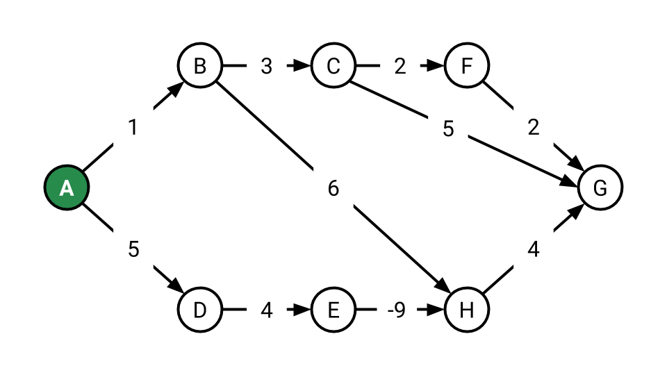
A valid topological ordering for this graph is A, D, E, B, H, C, F, G. If instead of considering edges ordered by their cost, we could consider them in its topological order; both A-D and A-E will be considered before considering A-B. Thus, we can reduce the problem of finding a shortest path in a DAG to a topological sort
for v in topological(G):
    for (w, weight) in G.neighbors(v):
        if distTo[w] > distTo[v] + weight:
            edgeTo[w] = v
            distTo[w] = distTo[v] + weight
In this algorithm, a vertex is considered only when all of its possible incoming edges have been processed.
What is the runtime of the algorithm?
O(V + E) for finding a valid topological ordering via reversing the postorder DFS traversal.
O(V + E) to consider every vertex and relax every edge in the graph.
This is also asymptotically faster than Dijkstra’s algorithm, which has a runtime in O(E log V) for E > V. However, this algorithm does not work on the graphs that contain cycles.