Graph Implementations Reading
Disclaimer: This reading might be confusing! We’ll go over these topics in the next lecture, so try to pick up as much as you can.
From CSE 143, you should be familiar with these 3 types of Tree Traversals: Preorder, Inorder, and Postorder. Here’s a reminder of what they look like. 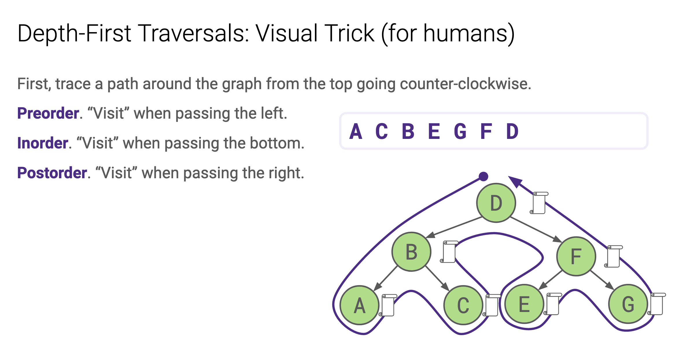
These are depth-first search (DFS) algorithms. In DFS, we visit down the entire lineage of our first child before looking at our second child.
Trees. A tree consists of a set of nodes and a set of edges connecting the nodes, where there is only one path between any two nodes.
Graphs. A graph consists of a set of nodes (or vertices) and a set of edges connecting the nodes. However, unlike our tree definition, we can have more than one path between vertices, known as a cycle. Note that all trees are graphs but not all graphs are trees.
Notice how this graph looks different than a tree. 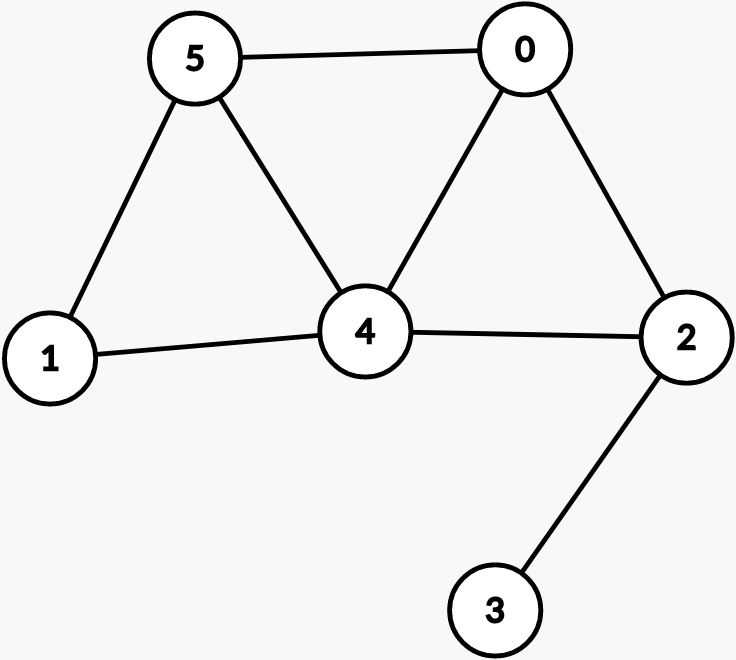
In this course, we can assume all graphs are simple graphs, which means they contain no self-loops or parallel edges. A self-loop is an edge that starts and ends at the same vertex. A parallel edge is a pair of edges connecting two vertices.
DFS on a graph needs to be slightly different than on trees. Since graphs may have cycles, and we don’t want to visit the same nodes more than once during a traversal, we need to check that each vertex should be visited at most once. This can be accomplished by marking nodes as visited and only visiting a node if it had not been marked as visited already.
Before discussing graph implementations, let’s introduce an important problem for motivating graphs. Given two vertices s and t, how can we determine if s and t are connected in our graph? In DFS, we start at a vertex and eventually visit every other vertex. So, we can start at s check if we encounter t at any point during DFS! In this example, s-t connectivity is a graph problem and DFS is a graph algorithm that solves it.
In the HuskyMaps project, we care not only about whether s and t are connected, but also the shortest path between s and t. One way to solve this problem on graphs is to use breadth-first search (BFS). In BFS, we visit every immediate neighbor before moving on, rather than visiting the first neighbor’s entire lineage like in DFS. This is similar to level-order traversal in a tree, which is where we visit every node on a level before going to a lower level. This way, we not only get the shortest path between s and t, but also the shortest paths from s to every other connected (reachable) vertex.
- Initialize a queue data structure (often called a fringe) with a starting vertex s and mark s.
- Repeat until the queue is empty:
- Remove vertex v from the front of the queue.
- For each unmarked neighbor n of v:
- Mark n.
- Set
edgeTo[n] = vanddistTo[n] = distTo[v] + 1. - Add n to end of queue.
edgeTo- A map for identifying the vertex v used to get to n.
distTo- A map for determining the distance from s to every other vertex n.
We set distTo[n] = distTo[v] + 1 because each unmarked neighbor n of v is one edge further away from s! If v is a certain distance from s, then n (a neighbor of v) is one more edge away from s.
In the upcoming lecture, we’ll take a slight detour to discuss graph representation problems, their relationship to graph algorithms, and how to actually implement them in a programming language like Java.