In this project, you are required to extend a spline-based animation system
to support multiple curve types, and implement a particle system simulation engine.
After building a working system, you will use your (robust and powerful)
program to produce a (compelling and arresting) animation.
The skeleton code provided extends on top of the same architecture as Modeler, and is designed so that you can re-use your models.
(Using your own model(s) is a requirement for this project, but you can make any changes to your previous model that you feel are appropriate, and can add new models that you've developed since Modeler.)
You can run Animator just like with Modeler and load your .yaml file via File->Open Scene.
Begin by pulling the Animator updates to your Modeler repo, and merging any conflicts that result. Do this early! If you find yourself having significant trouble with merging, go to office hours for help.
Note: Lights have been updated in Animator. If you added additional lights to modeler (such as spotlights) and want to use those in Animator, you'll have to write a GLRenderer::Render method for that light type. See the point light and directional light overloads of the Render method for reference. Then modify GLRenderer::Render(SceneObject& node) to call the method you wrote when rendering lights.
Animator uses the same interface as the Modeler application, with the addition of an Animation tab on the bottom window.
This window, along with the Inspector sidebar is where you'll be spending most of your time.
The Animation window is where you edit a time-varying curve for each model parameter by adding and moving control points (also known as keyframes).
Selecting controls from the left section of the Animation window brings up the corresponding curves in the graph on the right.
Here, time in number of frames is plotted on the x-axis, and the value of a given parameter is plotted on the y-axis.
This graph display and interface is encapsulated in the AnimationWidget class.
Requirements
Implement the features described below. The skeleton code has comments marked with // REQUIREMENT denoting
the locations at which you probably want to add some code.
Implement the following 3 curve types:
Bezier
They should be cubic beziers splined together with C0 continuity. You'll need at least four control points to make a single bezier curve. Adjacent Bezier curves share control points so that the last control point of one Bezier curve will be the first control point of another. In this way you can have two complete Bezier curves with only 7 control points and so on.
Note: In the lecture slides, you were shown an adaptive recursive algorithm for creating Bezier curves as well as a straightforward method that simply samples at a consistent rate. The adaptive Bezier curve generation is not required (but is a bell of extra credit). Feel free to sample the curve at a constant rate to fulfill the project requirements.
Catmull-Rom
Include endpoint interpolation.
Keep in mind that it is possible to make parametric curves that "double back" on themselves (x is not monotonically increasing as a function of t), which is obviously not desirable.
It must be possible to interpret the curves that your solution produces as a function of time, so you'll have to think about and solve this case when it occurs (for any curves).
B-spline
Include endpoint interpolation.
Create a particle system that:
Functions as part of the scene hierarchy
When you attach your particle system to a node other than the root, it should behave properly as a child of that node.
You'll have to think carefully about how to represent the positions of your particles.
Suppose you want to attach a particle shower to your model's hand.
When you apply the force of gravity to these particles, the direction of the force will always be along the negative Y axis of the world.
If you mistakenly apply gravity along negative Y of the hand's coordinate space, you'll see some funky gravity that depends on the orientation of the hand (bad!).
To solve this problem, you must operate in world space; particles' positions and velocities (and the forces that act on them) should be converted to world space by using the provided model_matrix_ field.
Has two distinct forces acting on it
The three most obvious distinct forces are gravity (f=mg), viscous drag (f=-k_d*v), and Hooke's spring law. Other interesting possibilities include electromagnetic force, simulation of flocking behavior, and buoyant force.
If the forces you choose are complicated or novel (or listed in the Bells and Whistles) you may earn extra credit while simultaneously fulfilling this requirement.
You must solve the system of forces using Euler's method.
Implements collision detection
You must detect and respond for two types of primitives that can be added to your scene:
Plane collision. A natural position for the plane is to have it act as the ground of your scene, but it could be placed anywhere. Planes have a width and height (not part of the Scale property).
Sphere collision. The sphere collision should be "natural" - i.e. the particles colliding with the sphere should reflect off the sphere dependent on the sphere's normal at the point of collision and the particle's incoming velocity direction.
Note that either primitive should be able to be moved and the particle collisions should collide with their current position, not just its original position.
Your particles should bounce off of the sphere and the plane, and the restitution constant slider should properly control how much the normal component of the reflected velocity is attenuated.
Animator Widget Interface
After selecting a model parameter in the tree on the left, the parameter's
corresponding animation curve is displayed in the graph.
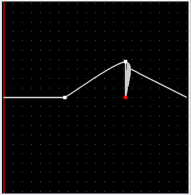
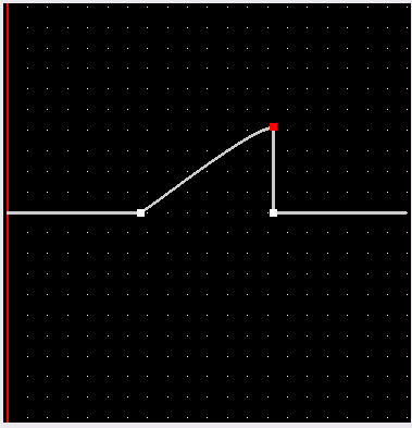
The skeleton evaluates each spline as a simple piecewise linear curve that linearly interpolates between control points.
Note that when you select a curve, it scales to the max and min value you have set as control points to "fit" into the graph window.
You can manipulate the curve as follows:
Command
Action
LEFT MOUSE
Selects and moves control points by clicking and dragging on them
SHIFT + LEFT MOUSE
Selects multiple control points
DRAG LEFT MOUSE
Rectangle-selects multiple points
DRAG RIGHT MOUSE
Pans the graph
SCROLL
Zooms the graph in X and Y dimensions
SHIFT + SCROLL
Zooms only the X axis (time in frames)
SHIFT + SCROLL
Zooms only the Y axis (parameter value)
F
Fits the graph view to the current control points
K
Creates a keyframe (control point) at the current time position
DELETE / FN + BACKSPACE
Removes the selected control point
At the bottom of the window is a simple set of VCR-style controls and a time slider that lets you play, pause, and seek in your animation. Along the menu bar of the Animation window, you can change a few settings:
Curve Type: Chooses how to interpolate between your control points, or keyframes. The skeleton currently uses linear interpolation for each, which you will have to fix (see below: Skeleton Code for Curves).
Wrap Curve: Interpolates between the last and first control points in your graph so that your motion can loop smoothly.
Linear curve wrapping is implemented for you; implementing curve-wrapping for the other curve types is a whistle of extra credit each.
Loop: Automatically loops playblack of your animation when it reaches the end.
Keyframe: Creates a keyframe (control point) at the current time position.
Set Length: Sets the length in seconds. NOTE: If you decrease the length of your animation, any keyframes that were set past that time length are deleted.
Set FPS: Sets the frames per second for playback of your animation.
Skeleton Code for Curves
The AnimationWidget object owns a bunch of Curve objects.
The Curve class is used to represent the time-varying splines associated with your object parameters.
You don't need to worry about most of the existing code, which is used to handle the user interface.
However, it is important that you understand the curve evaluation model.
Each curve is represented by a vector of evaluated points, calculated from a vector of control points.
std::vector<ControlPoint*> control_points_;
The user of your program can manipulate the positions of the control points
using the Animation Widget interface.
Your code will compute the value of the curve at intervals in time, determining the shape of the curve.
Given a set of control points, the system figures out what the evaluated points are based on the curve type.
This conversion process is handled by the CurveEvaluator member variable of each curve.
Classes that inherit from CurveEvaluator contain an EvaluateCurve function; this is what you must implement for the required curve evaluators: Bezier, Catmull-Rom, and B-Spline.
C2-Interpolating curves can be added for extra credit.
In the skeleton, only the LinearCurveEvaluator has been implemented, and each other evaluator currently acts as a linear curve.
Consequently, the curve drawn is composed of line segments directly connecting each control point.
Use LinearCurveEvaluator as a model to implement the other required curve evaluators.
CurveEvaluator::EvaluateCurve
This function returns a vector of the evaluated points and takes the following parameters:
ctrl_pts--a collection of control
points that you specify in the curve editor animation_length--the largest time, in seconds,
for which a curve may be defined (i.e., the current "movie length") wrap--a flag indicating
whether or not the curve should be wrapped (wrapping can be implemented for
extra credit)
For Bezier curves (and the splines based on them), it is sufficient to
sample the curve at fixed intervals of time. The adaptive de Casteljau
subdivision algorithm presented in class may be implemented for an extra bell.
Catmull-Rom and B-spline curves should be endpoint interpolating. This can
be done by doubling the endpoints for Catmull-Rom and tripling them for
B-spline curves.
You do not have to sort the control points or the evaluated curve points.
This has been done for you. Note, however, that for an interpolating curve
(Catmull-Rom), the fact that the control points are given to you sorted by x
does not ensure that the curve itself will also monotonically increase in x.
You should recognize and handle this case appropriately. One solution is
to return only the evaluated points that are increasing monotonically in x.
Also, be aware that the evaluation function will linearly interpolate
between the evaluated points to ensure a continuous curve on the screen.
This is why you don't have to generate infinitely many evaluated points.
Particle System Simulation
UI
The particle system as a whole, sphere colliders, and plane colliders have been added to the Animator UI as SceneObjects.
You may add them to your scene the same way you add 3D Objects, and their properties will appear in the right-hand Inspector window.
For particle systems, sliders are included for Period, controlling how often particles are emitted, and Restitution, the constant you should use in calculating collision force attenuation.
You'll also notice Sphere properties in the Inspector. The skeleton currently uses sphere primitives as the Geometry component for particles. If you'd like to change that, modify what component is added inside the Scene::CreateParticleSystem method.
Skeleton Code
The skeleton code has a very high-level framework in place for running
particle simulations that is based on Witkin's Particle System
Dynamics. In this model, there are three major components:
Particle objects (which have physical properties such as mass, position and velocity)
Forces
An engine for simulating the effect of the forces acting on the particles
that solves for the position and velocity of each particle at every time
step
You are responsible for coming up with a representation for particles and
forces. You will be computing the forces acting on each particle and updating their positions and velocities based on these forces using Euler's method. Make sure you thus model particles and forces in some way that allows you to perform this update step at each frame.
The skeleton provides a very basic outline of a simulation
engine, encapsulated by the ParticleSystem class within scene/components. The model_matrix_ field is provided for you to use in converting local coordinates to world space. The skeleton also already includes PlaneCollider and SphereCollider objects, but you will need to implement the collision detection code within the ParticleSystem class.
Note that the ParticleSystem
declaration is by no means complete. As mentioned above, you will have to
figure out how you want to store and organize particles and forces, and as a
result, you will need to add member variables and functions. If you want to provide further UI controls or more flexibility in doing some very ambitious particle systems, you can also search for how the interface is used and re-organize the code. Bells and whistles will be awarded for super cool particle systems, proportional to the effort expended.
Please follow the general instructions here. More details below:
Artifact Submission
You will eventually use your program to produce an animated artifact for
this project (after the project due
date – see the top of the page for artifact due date). Each group should turn in one artifact that they created together. We may give extra credit to those
that are exceptionally clever or aesthetically pleasing. Try to use the ideas
discussed in the John Lasseter article.
These include anticipation, follow-through, squash and stretch, and secondary
motion.
Camera Set-up: To create your animation, you'll need to go to SceneObject->Create Camera to add a render camera to your scene. The view from this camera is what will be rendered out when you save movie frames. Set properties like the Resolution via the right-hand Inspector window, and look through the camera by changing the view from Perspective to your Scene Camera via the scene's menu bar.You can manipulate the position and angle of the camera like any object (and you can also key it in the Animation window!), but not via controlling the view while you are looking through the camera. You may instead find it useful to open a New View and then have both view windows open, one in Perspective and one in your Scene Camera.
Timing: Finally, plan for your animation to be 30 seconds long (60 seconds is the
absolute maximum). We recommend dividing this time into separate shots, and saving a .yaml file for each. The .yaml file contains the spline curves you use for each model property, so you'll want to keep an original scene file to build off of when creating your shots. Plan out your animation - you will find that 30 seconds is a very small amount of time. We reserve the right to
penalize artifacts that go over the time limit and/or clip the video for the
purposes of voting.
Exporting: When you're ready, under the File
menu of the program, there is a Save Movie Frames option, which will let you
specify a base filename for a set of movie frames. Each frame is saved as
a .png, with your base filename plus some digits that indicate the frame number. Use a program like Adobe Premiere or Blender (installed in the labs) to compress the frames into a video file.
Refer to this Blender guide for
creating the final submission (an H.264 MP4 file). You can use different programs or play with the settings to produce different encodings for your own purposes, but the final submission must be an H.264 MP4.
Absolute
time limit: 60 seconds...shorter is better!
Animation
will count toward final grade on animator project.
The
course staff will grade based on technical and artistic merit.
You must turn in a representative image (snapshot) of your model/scene and your completed artifact (as a video) using
the artifact turn-in interface. See due dates/times at the top of this page.
Do not be late!
Important: Compile executable in Release Mode!
There is an increase in performance by compiling and creating your artifact in release mode vs debug mode. Also, Save As often, and create multiple shots! There is no undo button.
Bells and Whistles
Bells and whistles are extra extensions that are not required, and will be worth extra credit. You are also encouraged to come up with your own extensions for the project. Run your ideas by the TAs or Instructor, and we'll let you know if you'll be awarded extra credit for them. If you do decide to do something out of the ordinary (that is not listed here), be sure to mention it in a readme.txt when you submit the project.
Come up with another whistle and implement it. A whistle is something that extends the use of one of the things you are already doing. It is part of the basic model construction, but extended or cloned and modified in an interesting way. Ask your TAs to make sure this whistle is valid.
Enhance the
required spline options. Some of these will require alterations to the user
interface, which involves learning Qt and the UI framework. If you
want to access mouse events in the graph window, look at the CurvesPlot
function in the GraphWidget class. Also, look at the Curve
class to see what control point manipulation functions are already
provided. These could be helpful, and will likely give you a better
understanding of how to modify or extend your program's behavior. A
maximum of 3 whistles will be given out in this category.
Let the user control the tension of the Catmull-Rom spline.
Implement
one of the standard subdivision curves (e.g., Lane-Riesenfeld or
Dyn-Levin-Gregory).
Add
options to the user interface to enforce C1 or C2
continuity between adjacent Bezier curve segments automatically. (It
should also be possible to override this feature in cases where you don't
want this type of continuity.)
Add
the ability to add a new control point to any curve type without changing
the curve at all.
The linear curve
code provided in the skeleton can be "wrapped," which means that the
curve has C0 continuity between the end of the animation and the beginning. As
a result, looping the animation does not result in abrupt jumps. You will be
given a whistle for each (nonlinear) curve that you wrap.
Modify your particle system so that the particles' velocities get initialized with the
velocity of the hierarchy component from which they are emitted. The particles
may still have their own inherent initial velocity. For example, if your model
is a helicopter with a cannon launching packages out if it, each package's
velocity will need to be initialized to the sum of the helicopter's velocity
and the velocity imparted by the cannon.
Particles rendered as points or spheres may not look that realistic. You can achieve more
spectacular effects with a simple technique called billboarding. A
billboarded quad (aka "sprite") is a textured square that always
faces the camera. See the
sprites demo. For full credit, you should load a texture with
transparency (sample textures), and
turn on alpha blending (see this tutorial
for more information). Hint: When rotating your particles to face the
camera, it's helpful to know the camera's up and right vectors in
world-coordinates.
Use the billboarded quads you implemented above to render the following effects.
Each of these effects is worth one whistle provided you have put in a whistle
worth of effort making the effect look good.
Fire (example) (You'll probably want to use
additive blending for your particles -glBlendFunc(GL_SRC_ALPHA,GL_ONE);)
Add baking to your particle system. For simulations that are expensive to process, some
systems allow you to cache the results of a simulation. This is called
"baking." After simulating once, the cached simulation can then
be played back without having to recompute the particle properties at each time
step. See this page for more information on how
to implement particle baking.
Implement a motion blur effect (example). The easy
way to implement motion blur is using an accumulation
buffer - however, consumer grade graphics cards do not implement an
accumulation buffer. You'll need to simulate an accumulation buffer by
rendering individual frames to a texture, then combining those textures.
See this
tutorial for an example of rendering to a texture.
Euler's method is a very simple technique for solving the system of differential equations that
defines particle motion. However, more powerful methods can be used to
get better, more accurate results. Implement your simulation engine using
a higher-order method such as the Runge-Kutta technique. ( Numerical Recipes,
Sections 16.0, 16.1) has a description of Runge-Kutta and pseudo-code.
Implement adaptive Bezier curve generation: Use a recursive, divide-and-conquer, de
Casteljau algorithm to produce Bézier curves, rather than just sampling
them at some arbitrary interval. You are required to provide some way to change
the flatness parameter and maximum recursion depth, with a keystroke or mouse
click. In addition, you should have some way of showing (a debug print
statement is fine) the number of points generated for a curve to demonstrate
your adaptive algorithm at work.
To get an extra whistle, provide visual controls in the UI (i.e. sliders) to
modify the flatness parameter and maximum recursion depth, and also display the
number of points generated for each curve in the UI.
Extend the particle system to handle springs. For example, a pony tail can be simulated with a
simple spring system where one spring endpoint is attached to the character's
head, while the others are floating in space. In the case of springs, the
force acting on the particle is calculated at every step, and it depends on the
distance between the two endpoints. For one more bell, implement
spring-based cloth. For 2 more bells, implement spring-based fur.
The fur must respond to collisions with other geometry and interact with at
least two forces like wind and gravity.
Allow for particles to bounce off each other by detecting collisions when updating their positions
and velocities. Although it is difficult to make this very robust, your
system should behave reasonably.
Implement the "Hitchcock Effect" described in class, where the camera zooms in on an object, whilst at the same time pulling away from it (the effect can also be reversed--zoom out and pull in). The transformation should fix one plane in the scene--show this plane. Make sure that the effect is dramatic--adding an interesting background will help, otherwise it can be really difficult to tell if it's being done correctly.
Implement a "general" subdivision curve, so the user can specify an arbitrary
averaging mask You will receive still more credit if you can generate,
display, and apply the evaluation masks as well. There's a site at
Caltech with a few interesting applets that may be useful.
Perform collision detection with more complicated shapes. For complex scenes, you
can even use the accelerated ray tracer and ray casting to determine if a
collision is going to occur. Credit will vary with the complexity shapes
and the sophistication of the scheme used for collision detection.
If you find something you don't like about the interface, or something you think
you could do better, change it! Any really good changes will be
incorporated into the next Animator. Credit varies with the quality of
the improvement.
If you'd like, go back and implement any of the extra credit for Modeler in your Animator project. You'll receive half of the stated credit (so one whistle instead of one bell, etc.). Obviously, you'll only receive credit for features that you didn't originally implement for Modeler.
x2
If you implemented billboarded quads with transparent textures, you may notice issues with the alpha blending. OpenGL renders objects out in a certain order and for proper alpha blending, you must render out all opaque objects first before you draw any objects that have transparency, which should then be drawn from farthest to closest to the camera. Do this with your billboards for the additional two bells.
x2
Currently, the code makes a draw call for each particle in the system, which is really expensive. A more performant way of doing this is using "instanced rendering", which is rendering a single mesh more than one time using a single draw call. Draw Particle Systems using Instanced Rendering in glrenderer.cpp to see much better performance.
x2
Add flocking
behaviors to your particles to simulate creatures moving in flocks, herds, or
schools. A convincing way of doing this is called "boids"
(see here for a short flocking guide made by 457 staff, and here for a demo and for more
information). For full credit, use a model for your creatures that makes
it easy to see their direction and orientation (as a minimal example, you could show this with colored pyramids, oriented towards the direction in which the creatures are pointing). For up to one
more bell, make a realistic creature model and have it move realistically
according to its motion path. For example, a bird model would flap its
wings to gain speed and rise in the air, and hold its wings outstretched when turning or gliding.
x2
Implement a C2-Interpolating
curve. You'll need to add it to the drop-down selection. See
this handout.
x2
Add the ability to
edit Catmull-Rom curves using the two "inner" Bezier control points
as "handles" on the interpolated "outer" Catmull-Rom
control points. After the user tugs on handles, the curve may no longer be
Catmull-Rom. In other words, the user is really drawing a C1
continuous curve that starts off with the Catmull-Rom choice for the inner
Bezier points, but can then be edited by selecting and editing the
handles. The user should be allowed to drag the interpolated point in a
manner that causes the inner Bezier points to be dragged along. See
PowerPoint and Illustrator pencil-drawn curves for an example.
x3
An alternative way to
do animations is to transform an already existing animation by way of motion
warping (animations).
Extend the animator to support this type of motion editing.
x4
Incorporate rigid-body simulations into your
program, so that you can correctly simulate collisions and response between
rigid objects in your scene. You should be able to specify a set of
objects in your model to be included in the simulation, and the user should
have the ability to enable and disable the simulation either using the existing
"Simulate" button, or with a new button.
Monster Bells
Disclaimer: please consult the course staff before spending any serious time on these. They are quite difficult, and credit can vary depending on the quality of your method and implementation.
Inverse kinematics
The hierarchical model that you created is controlled by forward kinematics;
that is, the positions of the parts vary as a function of joint angles. More
mathematically stated, the positions of the joints are computed as a
function of the degrees of freedom (these DOFs are most often
rotations). The problem is inverse kinematics is to determine the DOFs of a
model to satisfy a set of positional constraints, subject to the DOF
constraints of the model (a knee on a human model, for instance, should not
bend backwards).
This is a significantly harder problem than forward kinematics. Aside from
the complicated math involved, many inverse kinematics problems do unique
solutions. Imagine a human model, with the feet constrained to the ground. Now
we wish to place the hand, say, about five feet off the ground. We need to
figure out the value of every joint angle in the body to achieve the desired
pose. Clearly, there are an infinite number of solutions. Which one is
"best"?
Now imagine that we wish to place the hand 15 feet off the ground. It's
fairly unlikely that a realistic human model can do this with its feet still
planted on the ground. But inverse kinematics must provide a good solution
anyway. How is a good solution defined?
Your solver should be fully general and not rely on your specific model
(although you can assume that the degrees of freedom are all rotational).
Additionally, you should modify your user interface to allow interactive
control of your model though the inverse kinematics solver. The solver should
run quickly enough to respond to mouse movement.
If you're interested in implementing this, you will probably want to consult
the CSE558
lecture notes.
Interactive Control of Physically-Based Animation
Create a character whose physics can be controlled by moving a mouse or
pressing keys on the keyboard. For example, moving the mouse up or down
may make the knees bend or extend the knees (so your character can jump), while
moving it the left or right could control the waist angle (so your character
can lean forward or backward). Rather than have these controls change
joint angles directly, as was done in the modeler project, the controls should
create torques on the joints so that the character moves in very realistic
ways. This monster bell requires components of the rigid body simulation
extension above, but you will receive credit for both extensions as long as
both are fully implemented.. For this extension, you will create a
hierarchical character composed of several rigid bodies. Next,
devise a way user interactively control your character.
This technique can produce some organic looking movements that are a lot of
fun to control. For example, you could create a little Luxo Jr. that hops
around and kicks a ball. Or, you could create a downhill skier that can
jump over gaps and perform backflips (see the Ski Stunt example below).
If you want, you can do it in 2D, like the examples shown in this paper (in
this case you will get full monster bell credit, but half credit for the rigid
body component).


