Further Reading - Topic 2 Roofline Model
 CSE 599M
Background
Roofline is a widely used performance model (simple yet effective in analyzing model performance), which can be summarized as:
\[P = \min\left\{\begin{eqnarray*} \pi \\ \beta \times I \end{eqnarray*}\right.\]where \(P\) refers to attanable performance, which will be measured by FLOPs/s (number of floating point operations per second).
The \(\pi\) refers to the maximum attainable FLOPs/s for the hardware, which is limited by the frequency/number of ALUs in the hardware, and we will explain this later.
The \(\beta\) refers to the memory bandwidth (bytes/second), which is also limited by hardware. The \(I\) is the operational intensity, which means the number of floating point operations we perform for each byte of data we fetch from memory, this value is determined by the algorithm.
If \(I\) is low, then even if the hardware has high peak FLOPs/s, the algorithm could not reach that performance because we are bounded by memory bandwidth, the compute units are waiting for data to come.
If \(I\) is high enough, and memory traffic is full, then the algorithm can fully utilize compute units in the hardware and we reach the peak performance.
Below is its visual explanation (source: Roofline: An Insightful Visual Performance Model for Floating-Point Programs and Multicore Architectures):
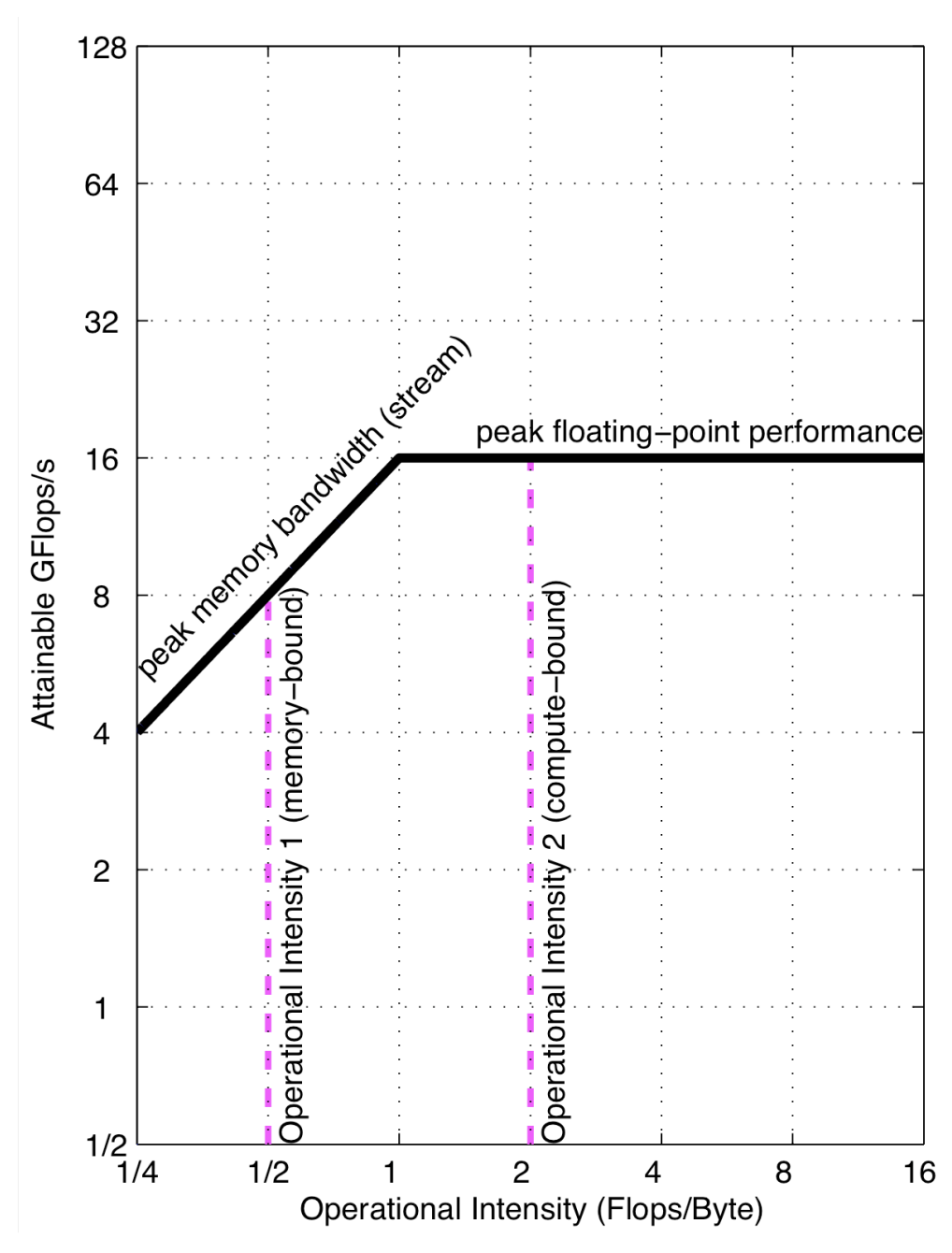
Where the x-axis refers to the operational intensity (FLOPs/bytes), and the y-axis refers to the attainable number, measured by FLOPs/s. The slope refers to the memory bandwidth.
The roofline is composed of a peak bandwidth ceiling (on the left side) and a peak performance ceiling (on the right side). The workloads on peak bandwidth ceiling is I/O bound and workloads on peak performance ceiling is compute bound.
Each generation of GPUs/TPUs would significantly increase the peak performance (ceiling height) by increasing the number of arithmetic units, however, memory bandwidth is harder to increase compared to peak performance, which is also known as memory wall. Clever implementation such as software managed scratchpad memory and prefetching technique can help us leverage faster memory, which makes the peak bandwidth ceiling higher.
Operators such as sigmoid have very low operational intensity (for each input element we only compute \(O(1)\) floating point operations) and operators such as matrix multiplication are preferable because of high operational intensity (each element in \(A\) and \(B\) (for \(C = A * B\)) will be multiplied and added with \(O(n)\) elements).
How to compute FLOPs
FLOPs of operators
On the software side, each floating point scalar addition/multiplication will count as a FLOP (floating point operation).
For example, if we are compute the dot product of two fp32 vectors with length 10:
import numpy as np
x = np.random.rand(10)
y = np.random.rand(10)
z = np.dot(x, y)
The FLOPs is 20, because the multiply takes 10 FLOPs and addition takes another 10 FLOPs:
z = 0 + x[0] * y[0] + x[1] * y[1] + ... x[9] * y[9] (there are 10 additions and 10 multiplies).
The FLOPs of a model is the sum of FLOPs of all operators in the model, there are many open source tools for computing FLOPs of a model (e.g. pytorch-OpCounter). The model FLOPs do not necessarily reflect real execution time, because it doesn’t consider whether we can reach the peak performance of the hardware, some operators has low operational intensity and will be bound by memory bandwidth, and some operators are irregular (e.g. Sparse NN) thus cannot fully utilize the hardware acceleration units. The RegNet claims that number of activations is a better proxy of running time than FLOPs.
FLOPs/s of hardware
For hardware, we use FLOPs/s to measure its peak performance, for a single chip it can be computed as:
\[\textrm{FLOPs/s} = \textrm{#cores} * \textrm{frequency} * \frac{\textrm{FLOPs}}{\textrm{cycle}}\]Let’s read the spec of NVIDIA A100 chip: there are 432 fp16 tensor cores, and the GPU boost clock for NVIDIA A100 GPU is 1410MHz. Each A100 Tensor Core can execute an 8x4x8 matrix multiplication, which is 8 * 4 * 8 * 2 = 512 FLOPs per cycle (the reason we multiply 2 is the same as the example of numpy dot product above, we need to count both multiplies and additions).
So the peak fp16 tensor core performance of A100 should be 432 * 1410 * 512 = 312 TFLOPs/s, which aligns with the A100 spec.
How to use the roofline model
The roofline model can help us identify the performance bottleneck of our workloads (whether it’s I/O bound or compute bound, but actually most of the workloads are I/O bound). Kernel fusion can help us remove lots of I/O intensive operators by computing them as an epilogue in compute intensitive kernels like matrix multiplication.
From the algorithm side, we can always modify the algorithm to increase the operational intensity, low operational-intensity models would no longer be used unless they demonstrate much better accuracy, and we are seeing Deep Learning models converges to a combination of different matrix multiplications operators.
Note that different hardware have different “shape” of roofline, and one model might be I/O bound on one hardware but compute bound on another hardware.