CSE 576 Computer Vision

Project 1 Feature Detection and Matching

Xinhang Shao

04/18/2013

1. Feature Detection

For feature detection, the method is exactly the same as the one in the project description. A 3x3 Sobel operator was used to calculate the x and y gradients. I also tried a simple one with Ix = I[x+1,y] – I[x,y] and Iy = I[x,y+1] – I[x,y]. It was not as good as the Sobel operator since the Sobel operator takes weighted average of six gradients and thus smoothes the difference a little bit. A 5x5 Gaussian mask was used to calculate the Harris matrix values according to the gradients. The Harris operator, which is the ratio of the determinant to the trace, gives the corner strength c at each pixel. The value c was multiplied by 100 to get better visualization of the Harris image. There are two requirements for a pixel to be a good feature: 1) its c value is local maximum in a 3x3 window; 2) its c value is above a threshold. The threshold is optimized for each input image. First, find the minimum and the maximum of c. The initial threshold level is 0.2, which means the threshold value = min + 0.2*(max-min). Next, count the number of features that satisfy the two requirements. If the number is larger than 1000, reduce the threshold level by half; if the number is less than 500, increase the threshold level by half. This iteration stops if the number of features is between 500 and 1000, or it iterates for 10 times. Usually, the number of iteration is less than 3.

2. Feature Description

Two kinds of feature descriptors are used.

The first one is a 5x5 window. It takes 25 pixel values centered at the current pixel on the converted gray image as feature descriptors.

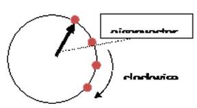
The second one is a circular descriptor. I referred to the reports of Spring 09, and found this idea very interesting. Actually that student got the first place, so why not? Instead of using a square window, the circular descriptor uses a circular window, and takes pixel values at the center of the circle (the current pixel), as well as at circumferences with r = r₀, 2*r₀, and 3*r₀, as shown in the figure below. Since MOPS extracts features from 40*40 raw data, so a reasonable guess would be r₀ between 5 and 8. Samples were taken at 20 degrees apart, starting from the dominant orientation. The dominant orientation was calculated from the eigenvector corresponding to the larger eigenvalue. The sample pixel was rounded to the nearest integer pixel, so a possible improvement is to use bilinear or cubic interpolation to get more precise values.

I tried r₀ = 5, 6, 7, 8 and 10, with step angle = 20^o or 30^o, and found that r₀ = 6 gives the best performance using the 4 benchmark sets of images. The performance was evaluated by summing up the average AUC of the four sets. Different images behave differently when r₀ changes. For the step angle, 20^o is better than 30^o by about 0.005 ~ 0.01 in terms of average AUC, and the tradeoff is more resources due to more data points taken. This sampling method makes the feature descriptors rotation invariant.

To get scale invariance, the original gray image were shrunk to 1/2 x 1/2 and 1/4 x 1/4 sizes by taking out every other pixel after low pass filtering by evenly weighted 3x3 mask. Other low pass filters could also be used.

For both descriptors, the values were subtracted by the mean, and then divided by the standard deviation of the descriptor, which makes them illumination invariant.

3. Feature Matching

Two matching methods were used. One was the given SSD method, and the other one was ratio test, which takes (distance of the best match) / (distance of the second best match).

4. Performance

(1) ROC

ROC of graf	ROC of Yosemite

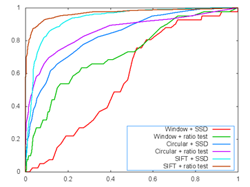
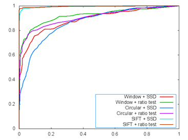
The ROC curves are mostly as expected except some for Yosemite, which surprised me that the circular descriptor was not better than the 5x5 window descriptor. Again, the 5x5 window descriptor I used was also illumination invariant.

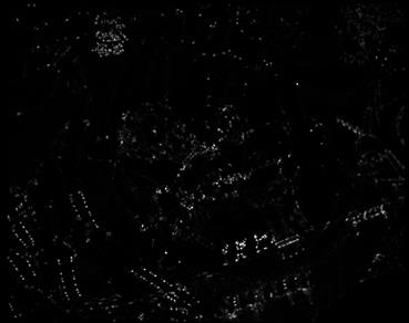
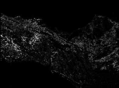
(2) Harris value images

The original values were multiplied by 100 to get better visualization.

Graf	Yosemite

(3) AUC

Below is a summary of the AUC of four benchmark sets. For the circular descriptor, r₀ = 6, step angle = 20^o.

	Window + SSD	Window + ratio	Circular + SSD	Circular + ratio
bikes	0.601972	0.617781	0.841025	0.894008
graf	0.563350	0.685072	0.718351	0.748482
leuven	0.725803	0.832564	0.858521	0.905749
wall	0.744245	0.767936	0.813687	0.802752

5. Strengths and Weaknesses

(1) My implementation is invariant to translation, which is the property of Harris features.

(2) It is illumination invariant, since the descriptors are subtracted by the mean and then divided by the standard deviation.

(3) It is rotation invariant, since values in the feature descriptors begin with the dominant orientation.

(4) It is scale invariant, since feature descriptors were created for three scales of the original images.

(5) Feature cluster is the biggest weakness of my implementation. In SIFT methods, features distribute evenly. In contrast, my features cluster at high frequency part, some of which are redundant. As for my circular descriptor, one pixel of interest could have at most three descriptors, which worsens the situation. A possible improvement of the 1-to-3 issue is suggested in the next section, but I did not have enough time to implement it this time.

(6) The sampling radii of the circular descriptor may affect image differently. Generally, small radius is better for high frequency features, and larger radius is better for low frequency features. It’s possible to optimize the sampling radii, but may take more resources, such as time and memory.

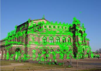
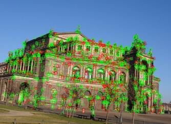
6. My Own Images

Here are my own images, showing rotation and scaling. Please note that for each pixel of interest, there are at most three feature descriptors with three scales. However, not all of them will match the three in the other picture. That’s why there seem to be a lot of mismatches. In the next step, we should combine three descriptors into one (store 55*3 pixel values), and implement another match method. That is, the match score of a pair of features is the highest of any 1/3 feature pairs. In this way, it eliminates any redundant feature descriptors, and will not show false mismatch in the given GUI.

Original Image	Rotation
Scale
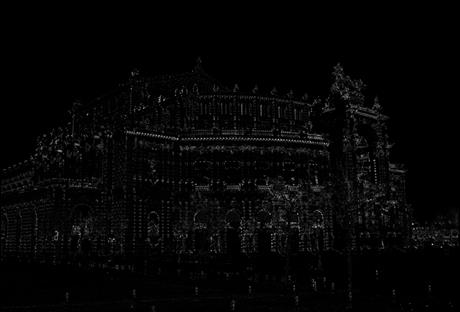
Harris Image

7. Extra Credits

(1) Implement the circular descriptor.

(2) The feature descriptor is scale invariant.