CSE 527 Lecture Note #13

Lecture: Prof. Larry Ruzzo

Note: Daehyun Baek

November 20, 2001

Bayesian Model Selection (BMS)

BMS is another way of doing notion of hypothesis A vs. hypothesis B to explain the data. The Bayesian information criterion(BIC) score is similar to chi-square value in the traditional hypothesis testing.

Bayesian Information Criterion (BIC)

: This is also an approximately statistical approach, not rigorously defined.

where D: Observed data,

M: Model (The Model is actually a family of models with unit variance and unknown mean therefore is needed),

: The maximum likelihood estimator (LME) of parameters in the model,

d : The number of free parameters, and

n : The number of data points.

Note: BIC score is good for comparing models. A model with a higher BIC is a better model, since if data fits well to the model, the log likelihood would be higher.

General model à Mixture model BIC with multiple models

BIC with multiple parameter estimators

Multiple parameters get higher likelihood but it is penalized by the second term (). If we mix two Gaussian parameters, becomes a pair. The likelihood will increase if there’re more model parameters. The second term, denotes a penalty term that also increases if more parameters are used. Intuitively, more data points need higher precision so it should be penalized.

Minimum Description Length (MDL) problem

Idea: Simpler is better. à Completely heuristic approach.

Let’s define M as a model, as a parameter (vector), and D as observed data.

: Bayes’ theorem

This is based on the 2-stage experiment. 1) Pick and 2) Draw data points according to . In this experiment, the above equation is a rigorous description of the model and denotes the posterior probability. It gives us a way to update the prior after seeing the data points D.

Idea: is the prior probability, which is subjective. Based on subjective belief, we can estimate , the distribution of given the data.

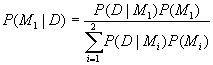
By the law of total probability,

(1) : Probability of data given the parameter

Suppose we have M₁, M₂, , and .

(2) : is the prior probability here.

Notice that is independent of . From (1),

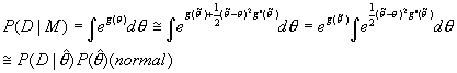
(3) : Integrated likelihood over the

parameter

Now,

: Posterior odds ratio

The odds ratio needed to establish data from which the model came becomes the following equation.

Posterior Bayes Prior

Odds factor Odds

Example of prior odds: Situation in a bath with mixed fair and biased coins.

Note that Bayes factor explains the favors of probability of data to the given models.

Thus, the goal here is to determine the posterior odds that is updating the prior odds after seeing the data as the data explains the model. Eventually, we want to estimate (3) because . However, the integral in (3) often is unsolvable in practice. So, let’s define as follows.

By Taylor series expansion, can be expanded as the below equation.

(4)

At the mode, . So the second term in (4) goes away. Therefore, (4) can be approximately simplified as follows.

Hint: The posterior mode would be close to the peak. The second derivative would be negative since there’s a convex near the peak. The width is related to one of variances in this distribution.

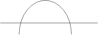
Width

Therefore, the second derivative term can be simplified. à

For multiple parameters

(By approximation not described here)

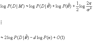
This concluded equation doesn’t have any prior probability term, which was omitted during the approximations by the assumption of unit information prior. The unit information prior is a proper assumption, when we are not sure about the prior probability.

Interpretation of BIC values: BIC difference of 10 favors one model over the other by the factor of about 150.

Approximations in this approach

1) Taylor series third and higher order expansions are ignored.

2) In the posterior distributions, the mode is observed to be near local maxima.

3) O(1) doesn’t go to zero if data set becomes bigger

4)

Covariance Model

: Covariance matrix for k_th cluster

, , and explain volume, orientation, and shape of the distribution, respectively.

Equal volume spherical model (EI): similar to k-means model

Unequal volume spherical model (VI)

More flexible,

but more parameters

Diagonal model: cluster shapes parallel to axes

where is diagonal,

EEE elliptical model: cluster shapes parallel to each other

Unconstrained model (VVV)

Bottom line: BIC allows to choose the best possible model whereas MLE will always favor VVV model. In general, VVV model is the best model in terms of the highest likelihood, however it needs larger number of parameters.