Interactable Fluid Simulations in VR

Introduction

As I stated above, I was really inspired by powder and the cool simulated environments you could create in it. Setting up some environment and allowing the underlying physics to run their course was something that I found very satisfying. Powder was only in two dimensions and I felt like adding a third would only serve to add to its immersion - and making it in VR would add even more while also being in the vein of the course. I was especially motivated since there were very few particle sims in VR. However, the simulation in powder includes many different particles and properties that would be very hard to implement in the little time I had so I chose to focus only on simulating water - still a difficult task but there was at least a lot of existing literature on this topic. I some experience with Unity and I knew Unity had great VR support so I opted to implement this project using it.

Related Work

Realistic fluid simulations are no new thing. One of the most cited papers on fluid simulations as I am implementing is Zhu and Bridson's 2005 paper "Animating Sand as a Fluid." They present very detailed explanations of their method of fluid simulation that combines the strengths of grids and particles. Matthias Müller recreates this method in an extremely helpful youtube video which describes the FLuid Implicit Particle. He also provides source code for implementing this method in two dimentions. David Li implemented a 3D interactable fluid simulation online which greatly inspired my own work. Macklin and Müller's 2013 paper "Position Based Fluids" offers another fluid simulation that also served to inspire my work. Nvidia's Cataclysm FLuid Implicit Particle solver with GPU Particles also inspired me, though implementation details were missing. Simon Green created a very helpful guide, "Screen Space Fluid Rendering for Games," which documents a method for rendering particle based fluid simulations in a realistic way - I had hoped to implement this as well, but could not due to time.

I used the same math as the related work above as I do not have time to implement my own unique fluid solver as cool as that would be. I only had access to Müller and Li's implementations from the work listed above, but my implementation still was unique in the following ways: I implemented the rendering of particles using Unity's GPU instancing, I made my simulation work in VR for real time VR interactions, and I solved all of the simulation in parallel with shared compute buffers and compute shaders. My implementation being in VR as well as my need for parallel solvers also meant the algorithms I used needed to be updated slightly from the ones in the related work, but they are overall the same.

Contributions

The follow are my major contributions:

• I made an implementation of the Fluid Implicit Particle method for fluid simulations that runs in parallel and renders using GPU Instancing which result in a very fast simulation.
• I am publishing all of this code on GitHub for people in the future to reference when making their own fluid solvers.
• I made this simulation work in VR by modifying my rendering shaders to work in stereo.

Method

There are two typical ways fluids are simulated in 3D: Eulerian grids and Lagrangian particles. Eulerian methods keep track of variables on a fixed grid, and Lagrangian store fluid variables on individual particles. Zhu and Bridson [2005] discuss a method that combines the strengths of a grid based and particle based simulation: the Fluid-Implicit Particle (FLIP) method. In the FLIP method, particles in the simulation store their position and velocity, and exist in an underlying grid where cells keep track of their incoming/outgoing velocities, pressures, etc. At a glance, one step of the algorithm I implemented is as follows:

• Particles will integrate themselves according to their stored velocity and position.
• Each particle checks if it falls outside of the boundary, if so, then it will move back inside and set its velocity to 0.
• Every particle will perform a weighted transfer of its velocity to nearby grid cells based on its distance to these cells.
• We will solve for incompressibility of the grid cells. Since we are modelling water, we need to preserve water's property that it does not compress easily. I.e. we cannot allow more water to flow into a cell than flows out.
• Transfer the cell velocities back to particles within them.
• Finally we can color the particles based on their velocity, relative cell pressure or some other metric to create a more stylized simulation.

Ideally, all of these steps will be done in parallel, one after the other - using the same shared compute buffer on the GPU to minimize any expensive transfers of memory from CPU to GPU.

As for rendering, I used GPU Instanced rendering which is provided by Unity. So every particle used the same exact mesh for rendering - a simple sphere. Then color and position of the spheres would be determined by another parallellized function in my compute shader. Doing this rendering in VR requires a small change to the shader for our particles so that they are drawn in stereo - but this along with more details for the specifics of this implementation will be documented below.

Adding user interaction is trivial, thanks to how fast the simulation runs. All that's needed for user interaction is to track some sort of input in real time - a mouse in 2D, or a VR controller in 3D. Map this position to a position in the grid. Then, for every loop of the simulation, track the difference in its position, calculate the velocity based on this difference and the time passed, and finally add this velocity to nearby grid cells before solving for incompressibility.

Finally, to render the fluid more realistically, I wanted to use screen space fluid rendering. This involves taking the image of the fluid that is displayed on the screen, and performing some shader passes on this 2D image to make it appear more realistic for a viewer. However, as I stated above, I did not have the time or knowledge to implement this, though (details as I understand them) will be presented below.

Implementation Details

Put in all the specific implementation details here, including both hardware and software aspects. Even if you didn't build a piece of hardware, make sure to document what hardware you used, including your headset, computing environment, and major software libraries. If you implemented specific hardware devices, describe how you decided on the design parameters for the hardware. For example, if you built a VR headset, you'd apply the equations you previously introduced in the method section to decide on the values you used in your construction. If you implemented an algorithm, such as volume rendering, then you'd describe the function implementation details here (e.g., GitHub projects you built on, libraries you used, or specific aspects you found challenging and how you resolved them).

We will discuss the more specific implementation details of this project in parts (a few of the simulation steps are presented as videos at the top of the website):

Hardware/Software

To begin, I implemented all of this code on my personal computer which has an NVIDIA graphics card. The simulation was built in Unity version 2022.2.6f1 in the Universal Render Pipeline with the Mathematics package, Occulus XR Plugin and XR Interaction Tools package. All of the VR simulations were recorded using an Occulus Quest 2 provided by the class.

Code Organization

I had two main files for my code: A compute shader which has functions for each step/sub-step of my fluid solver and a C# script to set things up and run an Update() loop which in each loop will call the functions defined in the compute shader. The C# script is where parameters for the simulation are defined before each run. E.g. the simulation height, width and depth, the time step size, the particle radius, number of grid cells, etc. In the start() function, the C# script will calculate the number of particles and grid cells based on these input parameters and initialize a number of fixed length compute buffers that the compute shader will make use of. It is also important to release these buffers on disable as well. The C# script is also responsible for controlling the camera and any VR inputs that might take place.

Fluid Simulation

This is where the bulk of the project is centered. As stated in the introduction, I am implementing the FLIP method for fluid simulations. In this method, we maintain a large buffer of particles and grid cells.

Particles

The particles keep track of their position and velocity in two separate float3 buffers. So for example, $${ParticlePositions[i] = float3(a, b, c)}$$ which tells us that particle i is located at x = a, y = b, and z = c in whatever coordinates we are using. The velocity buffer acts in the same way.

Grid Cells

We will be using the marker and cell (MAC) method which discretizes the environment of our fluid simulation. And becase we have a discrete number of grid cells in each cardinal direction we can easily index them. Firstly we need to define how large our simulation space is - for this sim I typically chose a width of 40 unity units, and a height and depth of 20 unity units. Now, we define how "dense" we want to pack these unity units with cells. The more dense, the smaller our particles will look, but the slower it will run. Let's call the number of cells in the x, y, and z direction numX, numY and numZ respectively. If we have a grid cell at (i, j, k), then we can find its index as follows: $${index = i * (numY * numZ) + j * (numZ) + k}$$ In other words, we iterate over grid cells in the z direction first, the y second, and the x last. We will have buffers to keep track of grid cell velocities which behave the same as the buffers we had for particles. But we also will keep track of things like cell pressure, and cell type. We can define cell type for each step of the simulation by iterating over every particle and marking the cell it occupies as a fluid cell. That way, when we later need to iterate over our cells, we will only process the ones with fluid in them, which saves a lot of computation - this is the general idea behind a MAC grid.

Integrate Particles

This step is pretty trivial. We will simply update each particle's position by its velocity and the time step from the last iteration. We also will add gravity to the vertical velocity component in this step before we integrate.

Transfer to Grid Cells

Once all of the particles have moved to their new positions, we will transfer their velocities onto our grid. This will be done using a standard bilinear interpolation from the particle to the neighboring 4 cells. Or in 3D it will use trilinear interpolation on 8 cells. We will weight the velocity added to a cell based on its distance from a cell, determined by our interpolation. This addition will take place in the compute buffer for our cell's velocities. We will also add the weight to a different buffer for the cells. 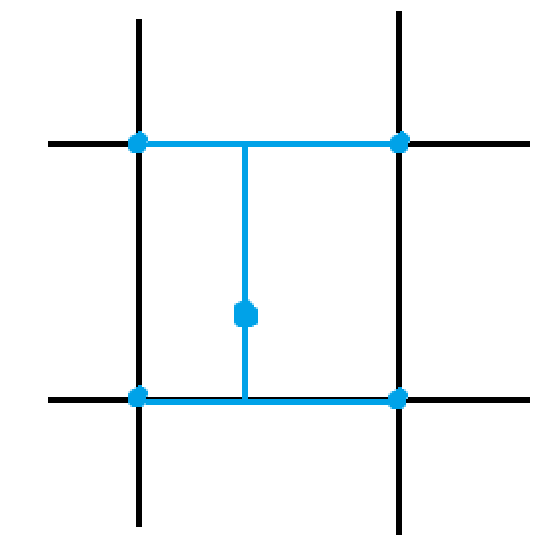Once we finish looping over all of the cells, we will divide the total velocity for each cell by the total weighted distance. Below is a simple diagram of a bilinear interpolation from a particle to the cell coordinates near to it. In order to find the cell a particle occupies, we will take its position and divide it by the height/width of a cell, which is determined when we initialize our grid. So for a particle at (x, y): $$x_{cell} = {\lfloor {x \above 1pt cell width} \rfloor}, y_{cell} = {\lfloor {y \above 1pt cell height} \rfloor}$$ However, since we are weighting this addition based on the distance from the cell velocity, we need to note the physical location of a cell's velocity. Consider the scheme used for storing a cell's velocity below: 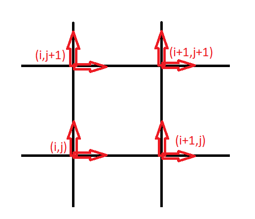However, we want our velocities to be positionally located at the cell faces like so: So the x velocity for cell (i,j) is positionally located at (i, j + 0.5*height), and the y velocity is positionally located at (i + 0.5 * width, j). So therefore, when we are trasferring a particles velocities to nearby cells, we need to account for this offset. When trasferring the x velocity of a particle, before we find the cell it occupies, we will offset its y value by -0.5 * cell_height, and when trasferring the y component, we will offset the x by -0.5 * cell_width. This has the side effect of requiring one extra row/column of the grid, but these correspond to cells outside of our grid, so we can simply ignore them after the transfer.

This transfer is very straight forward to implement iterativly, but in parallel we need to consider any race conditions that can occur. Like what happens if two particles are imbuing their velocities to the same cell components? In this case, we need to make sure we have memory safe adds. Luckily, we can use the existing Interlocked.Add method for memory safe adds. However, we want floating point precision for our simulation, but this function only support memory safe adds for integer types. We can work around this by multiplying our velocities by a large number (like 100,000) and then converting all of our velocities to ints and adding them. Then when we have transferred all of our particle velocities to cells, we can divide the result by the same number we scaled it by originally. This loses some precision, but in practice the simulation still worked.

Solve for incompressibility

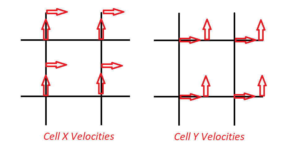
I've mentioned it before, but in order to make the fluid seem like a fluid, we need to make sure that the total flow into a cell is the same as the total flow out of a cell. From the diagram above, we can see that for some cell (i,j), the flow into a cell in the x and y direction is simply stored at the (i,j) index in our cell velocity buffer. Then, the flow out of this cell in the x direction is stored in the cell to the right, (i+1,j), and the flow out of the cell in the y direction is stored in the cell above, (i,j+1). We can compute the divergence, which is the total outflow from the cell as follows: $${divergence = xvelocity(i+1,j) - xvelocity(i,j) + yvelocity(i,j+1) - yvelocity(i,j)}$$ Intuitively, if there is a positive divergence, there is too much outflow, and if it is negative there is too much inflow. Ideally, we want the divergence for all cells to be 0. To make the divergence 0, we modify each of the velocities by the same amount: $${divergence \above 1pt 4}$$ So we will add this amount to the inflow values, xvelocity(i,j) and yvelocity(i,j), and subtract it from the outflow values, xvelocity(i+1,j), yvelocity(i,j+1). However, if the current cell is next to a wall, or other solid cell, we will NOT add any changes for the value that is adjacent to this wall, and only divide by the number of neighboring non solid cells when calculating this update rather 4.
We can solve this for all our cells by iterating over all fluid cells and performing these calculations for every one for a number of steps until convergence (though I just chose 100-1000 interations in practice). However, notice that this would be an iterative method, and our code is meant to be in parallel. I solved this by creating a new buffer, adding all of these updates for the cells to this buffer, and at the end of every iteration of my loop, add these values back to the grid and then perform the next loop. I used the same float to uint conversion as noted above. This probably isn't correct? But it worked in practice so I'm happy with it.
These implementation details are also all very informal - so I apologize, please look at my code or the references below for much better explanations.

Transfer back to particles

This is very similar to the step for going from particles to the grid. We will loop over every particle in parllel and find the cell it occupies using the same offset method we discussed above. We will again use bilinear/trilinear interpolation to find the nearest neighbors and then do a weighted sum of the velocity values for each cardinal direction and adjust the particle velocity by them. Note, that if a neighboring cell has no velocity, or is a solid cell, do not consider it in the weighted sum. Then, we need to consider how we want to add these velocites back to the particles. If we simply set the particle velocity to the weighted sum of the cell velocities near it, then a lot of the variation in velocity that particles have will be lost. So any particles that are in the same general area will all behave about the same and the fluid will end up looking viscous. This is actually called the Particle-In-Cell (PIC) method and it looks like this:



If we instead choose to add the DIFFERENCE between the previous cell velocities and the new velocities to our particle velocities, we can preserve a lot more variance in the simulation. This is what FLIP is and it looks like this:



It's a lot more noisy. We can actually combine these two methods for much better results. We can set the new velocity of our particles to a fraction of the PIC calculated velocity plus a fraction of the FLIP calculated velocity. In practice, it is chosen to use a FLIP fraction of about .9 and a PIC fraction of about .1. This combined method is usually referred to as PIC/FLIP and looks like this:

Rendering

The rendering implementation is a lot more code heavy, so I will mostly just refer to the code I used for these parts.

GPU instancing

I made use of Unity's built in Graphics function, DrawMeshInstancedIndirect to draw the particles on each step. I have a function in my compute shader which sets up the argsbuffer for this draw call. It will iterate over every single particle and update a different buffer filled with the properties for each particles rendering information. Specifically, it will update a transform matrix for each particle as well as a color based off of the density of the cell the particle occupies. Instanced indirect

Bringing the simulation to VR

When I first ran my code on my headset, I only rendered the scene onto one eye. Well, it rendered the scene to both eyes, but only the left eye got to see the particles. This is because the instanced shader I implemented did not have support for Single-pass instanced rendering which is how you can support stereo rendering for VR. I can't really explain this part, so please refer to this documentation.

Screen Space Fluid Rendering

I failed to get screen space fluid rendering working for this project. The idea behind it is to recreate the fluid's surface in screen space and apply some shaders to make it look like water. There is as lot more detail in presentation.

Evaluation of Results

This section should evaluate the benefits and limitations of your approach. Ideally, these should be quantitative details. If you implemented a foveated renderer, then you'd include measurements of frame time and image quality (e.g., PSNR). If you implemented a piece of hardware, then you'd want to show photographs of the results. Make sure to not just record successes here, but to also document limitations and failure cases. Show where your algorithm works and where it needs improvement. If you ran a user study, then you'd tabulate the statistics in this section and try to make some conclusions, based on that data. Ideally, if you had time to implement prior methods, you should include quantitative comparisons to the most promising related work you reviewed.

This wasn't the most quantitative project out there. When I start a simulation, I will instantiate all my particles in a square or something similar. So for most of my testing, I did a "Dam Break" simulation where I would instantiate all of my particles in a large block on one side of the sim and let them crash into the other side. Here's an example of a Dam Break with 175k particles on a (20,10,10) grid running at about 45 fps:



And adding the alpha blending doesn't seem to reduce any performance:



Here's an example of the sim running 625k particles at around 12.5 fps:


I think this looks amazing, but it just isn't possible to have real time interaction with a sim this large.

Running the simulation in VR was a lot slower. I think this is due to the stereo shader? It had to render twice the particles, one for each eye, but I felt like this should be faster. I could run a sim of size (10,5,5) with 100k particles at around 30-40 fps.



The sim above still very response and fast to interact with, the freezing of the "hand" is due to the lower battery life of the controller at the time of recording. If I try to render a similar sized sim to the one without VR, it will run at about 15 fps which is just not possible to have in VR:



And while it doesn't show up here, on the headset, there is terrible blending and warping of the images, which I imagine is due to the very slow fps.

In non VR mode, I also tested other starting configurations. The different starting positions did nothing for impact performance, but they look really cool so I'll add them here. Like a Double Dam Break:



A falling situation, not sure what to call this lol



This one actually highlights a bug in my implementation. Notice how the water tends towards the z = 0 axis as it falls. I'm not sure why, by my simulation likes to tend things towards z = 0 ever so slightly. I am not sure why, and it's hard to tell in other examples, but it really pained me for a while when I tried to fix but for time constraints, I left it in since it still looks cool.

There were other issues too. I constantly had to tweak the resting pressure of the simulation or else it would just break. For example, if I left the pressure too low the following would occur:



Or if it was too high:



Or if I did not include any damping when I imbued cell velocities to particles:



This is what most of my simulations looked like for a while - I did not figure out to add damping for so long.

And the most nefarious bug was this line of separation that exists near the y = 0 axis:



This actually occurs on both the x = z = 0 axis as well, but it only appears here because gravity forces the particles to the y = 0 one. I think this is due to the face that neighboring cells are the right, upper, or "deeper" cells, so when solving for incompressibility, the bottom cells dont have a neighbor from below to push them up? So they just want to lay on the bottom... I don't know, other FLIP solvers manually separate particles, but implementing this separation in parallel is a bit above my skill level and time so I left it!

There also is one elusive bug where the entire sim will bounce up like its jumping for joy. I couldn't record it, but I think it's due to the fact that my delta time for each simulation step is based off of the delta time in unity, and potentially something causes there to be a large spike between frames. Maybe my computer is processing something else at that exact time which causes the delta time to spike which causes everything to jump? Unsure, but it rarely bothered me.

Finally, I attempted to make screen space fluid rendering work, but it was so hard due to Unity's weirdly confusing rendering pipeline. I had little experience with shaders and implementing this turned out to be a bit too much in too little time. I don't have any decent results - the furthest I got before tapping out was implementing a gaussian blur on a render texture of the particle normals:



My setup was very scuffed - I had a camera rendering a render texture of the simulation with normals attached to the spheres. Then ANOTHER camera pointing at the render texture which was applying a blur. I would have kept going by implementing a bilateral blur, but I needed to get the depth texture of the image - for some reason, I couldn't grab this in a render texture in Unity. I'm sure there's a single line of code I was missing, but for the life of me I couldn't find it. So for the sake of my sanity and hairline, I chose not to continue.

Future Work

I really did not do anything ground breaking with this project. I implemented someone else's math in Unity's defined rendering pipeline - so I don't feel I have any ground to comment on future work for the field of fluid simulations. HOWEVER, I do have quite a bit of future work for this sim in particular. I need to address the bugs I listed above before I would be comfortable calling this project done. I left them in for the sake of time for this report, but all of them take away from the visual pleasure of my simulation. I also want to add some more complicated environments. Right now the fluid simulation takes place in a simple fish tank, but it would be cool to see this water navigate a maze or some other object. More methods of interaction in VR would make the simulation a lot more novel. One feature I am adding now but will not make it in the report is the ability to rotate the tank. So when the user picks up and rotates the tank, gravity will effectively change and the particles will fall to a new direction. And of course, I really wanted to add screen space fluid rendering to make the simulation look more like actual water - this is my biggest todo.

Conclusion

I had a lot of fun with this project. The purpose of this project wasn't to invent anything new, but to learn about fluid simulations and implement one in Unity. I feel like I accomplished that. In the future, I really want to work more with physics simulations and VFX in general since they're just so darn cool to look at. I think that these cool effects would be valuable in the VR space - the medium of VR/AR makes experiencing these effects a lot cooler. I really don't know what to type here.

Acknowledgments

This section is for thanking key collaborators that didn't do enough to warrant being a co-author of the paper. If someone financially sponsored your work or mentored you, then it's a good idea to recognize that here. If someone provided really helpful feedback or a great insight, then recognizing that contribution can be done here.

I could NOT have done this project without the help of some industry members:

• David Li implemented an amazing fluid simulation here. I reached out via email and he was extremely helpful by giving me a lot of high level understanding and resources on how fluid sims work.
• Olivier Mercier helped me attempt to implement the screen space fluid rendering for the last part of this project. While I did not succeed, Olivier was extremely helpful and nice.
• Douglas Lanman was my teacher for this course and was extremely supportive throughout this project. He helped me first decide what I was even going to do and also helped me brainstorm quite a bit.
• John Akers was like an assitant teacher for the course? Idk. He helped so much with setting up VR for this project, and was the main person I would bounce ideas off of.

Again, thank you to everyone who helped, even if you're not listed here.

References

My sources in no particular order. I know for a real report you need to cite them throughout the report and whatnot - but I got really lazy sorry :P.

• Yongning Zhu and Robert Bridson. 2005. Animating sand as a fluid. ACM Trans. Graph. 24, 3 (July 2005), 965–972. https://doi.org/10.1145/1073204.1073298
• Spencer, M. 2023. How to render 13,086,178 objects at 120 fps, YouTube. Available at: https://www.youtube.com/watch?v=6mNj3M1il_c
• Matthias Müller. 2022. 18 - how to write a flip water / fluid simulation running in your browser.
• Simon Green. 2009. Screen Space Fluid Rendering for Games. Availible at https://developer.download.nvidia.com/presentations/2010/gdc/Direct3D_Effects.pdf
• David Li. 2016. http://david.li/fluid
• Robert Bridson. 2008. Fluid Simulation for Computer Graphics second edition.
• Matthias Müller and Miles Macklin. 2013. Position based fluids. ACM Transactions on Graphics Volume 32 Issue 4.