Project 3: Trace
| Assigned | February 10th |
| Due | February 24th |
| Artifact Due | March 1st |
| Help Sessions |
1:30 pm February 12th |
| Project TA | Dalton Hildreth |
| Artifact Turn-in | |
| Artifact Winners | Winners |
 >
>
| Assigned | February 10th |
| Due | February 24th |
| Artifact Due | March 1st |
| Help Sessions |
1:30 pm February 12th |
| Project TA | Dalton Hildreth |
| Artifact Turn-in | |
| Artifact Winners | Winners |
 >
>
Trace is a program that constructs recursively ray-traced images of fairly simple scenes. It is similar in functionality to the POV-Ray raytracer. You may want to browse around the POV-Ray web site for artifact and extra credit inspiration. POV-Ray is free, so if you want a taste of what a really powerful raytracer can do, go check it out!
Visit here for help checking out code.
Inside the skeleton code, there is a "Editor/assets/trace" subdirectory which contain sample scene files (all the files with the .yaml extension). These are text files that describe some geometry and the material that should be applied to them. Load a scene and you'll be able to see the helpful debug view on the right. Go to [Render -> Raytrace Frame] to see the rendering.
Before you begin coding, you should run the sample solution; it is linked to on the right. It has all of the requirements implemented, along with some extra features. Definitely try clicking on the rendered scene and then check out the scene view in the UI to see how the ray travels in the space. It will help you a lot in debugging your ray tracing implementation!
The Trace project is a very large collection of files and object-oriented C++ code. Fortunately, you only need to work directly with a subset of it. However, you will probably want to spend a bit of time getting familiar with the layout and class hierarchy at first, so that when you code, you know what classes and methods are available for your use.
The starting point for where ray tracing begins, and where you will need to add a lot of functionality, is in the trace/raytracer.cpp file. This is a good file to start studying and exploring what methods get called and what they do. In addition, the raytracer features debugging inside the scene view that allows you to see individual rays bouncing around the scene. This window provides a lot of visual feedback that can be enormously useful when debugging your application. Look at the help slides (on the right) for a more detailed explanation of how to use the debugging window.
Implement the features described below. The skeleton code has comments marked with // REQUIREMENT denoting
the locations at which you probably want to add some code, and some further explanations.
After running the sample solution, you should build the skeleton code and see how it compares. You will probably notice that there is a significant difference in the quality of images rendered with the two versions. This suggests what parts of the raytracer have been written and what parts are left undone.
If you compare the outputs of the skeleton and solution, you will see that most of the basic geometry-handling code is done. The skeleton code is able to cast rays into an image and draw color on the screen, resulting in some flat-shaded polygonal shapes. The skeleton code is doing ray-casting and nothing more. Furthermore, any triangle and sphere primitives will not appear. While all the code to cast a ray exists, not all of the object intersections code is there. You need to implement sphere and triangle intersections and expand ray-casting into ray-tracing by adding support for reflected and refracted rays. You also must implement the Blinn-Phong specular-reflection model and include support for color-filtered shadows cast through transparent objects.
Specifically, everyone must implement recursive ray tracing as described in class. This entails making the extensions to the program listed below. Your ray tracer should recursively trace rays to account for these. Recursion should proceed to a maximum depth as set by the user.
Implement intersections in scene/components/sphere.cpp
See lecture sides or Marschner Shirley Handout 4.4.1
Note for the case of shere, you only need to compute the intersection point (i.t) and the normal (i.normal). UV is not a requirement, but worth 1 whistle if you implement it.
Fill code in Sphere::IntersectLocal() in scene\components\sphere.cpp
Implement intersections in scene/components/triangleface.cpp. See the Triangle-Intersection handout to get the equations you need.
For more details, please refer to Marschner Shirley Handout 4.4.2.
Fill code in TriangleFace::IntersectLocal() in Scene\components\triangleface.cpp
Fill code in TriangleFace::IntersectLocal() in Scene\components\triangleface.cpp
Normals (a.k.a. Phong interpolation)
Texture coordinates (uvs) if they exist on a trimesh
Note: When calculating the intersection for triangles, you may have 3 values for the normal (one for each vertex). You will have to interpolate these values in order to get the proper value. Don't forget to renormalize the interpreted normal! If the normal is not available, you may assume that it is just the normal used in the intersection calculation, i.e., the normal to the plane that the triangle lies in. If the vertices have texture uv coordinates, you will have to interpolate these to get the correct texture coordinate.
See lecture slides. You can also find shading equation in the note (Note: in the note, kr should be ks in our case).
From multiple light sources
Distance attenuation
Directional lights
Take a look at scene/components/light.h
See lecture notes
Objects blocking light sources
Color-filtering through transparent objects
(Implement filtered transparency as discussed in class)
See Marschner Shirley Handout 4.7
See the note to know how to derive reflection direction. Also See Marschner Shirley Handout 4.8 to get further details.
See the note to know how to derive refraction direction.
Be sure to handle the phenomenon of total internal reflection.
For further details, see Marschner Shirley Handout 13.1
(Ignore Fresnel term and Beer's Law, which are whistles)
You may assume that objects are not nested inside other objects. If a refracted ray enters a solid object, it will pass completely through the object and back outside before refracting into another object. Improving your refraction code to handle more general cases such as a refractive sphere contained inside another refractive sphere is an extra credit option as described below. In addition, you may assume that the camera itself is not placed inside an object. The initial rays that are sent out through the projection plane will always be moving through air.
Implement antialiasing by supersampling (send multiple rays) and then averaging down.
The dragon.yaml is a good scene to test this on!
See lecture notes
To enable auti-aliasing to verify your implemetation, click RenderCamera on the scene panel, and on the right inpector panel, change Samples Per Pixel to more than 1. More samples you set, more computations you will need to trace the scene, but also reduce more aliasing.
For this project, you are not required to implement any bells or whistles. At this time, we hope that you are already in the habit of thinking about extra features when you start the project. Even the simple bells and whistles can make significant changes in your ray traced scenes.
Recall how a raytracer functions, as described in class. The raytracer iterates through every pixel in the image, and, using some illumination model determines what color intensity is assigned to the pixel. The skeleton code goes through several functions to do this, but the real interest occurs when you get to the RayTracer::TraceRay( ) function. This is also where a handy diagram can start to be of help (shown below). The diagram is supposed to represent the flow of the ray tracing program. Each separately colored box represents a different function that you will have to add some code to in order to finish the project.
The traceRay function takes three arguments: a ray that needs to be traced, a threshold vector, and an integer that controls the depth of recursion for the ray tracer. It returns a color (represented through a three-dimensional vector). The signature of this function should make its purpose clear: a ray is input to it, and the function determines the color that should be projected back to whatever it was that cast the ray. In order to do this, the first thing traceRay wants to know is if the ray actually hits anything that is worth looking at, or if it wanders off into the lonely darkness of space. This is where a test for ray/object intersection occurs (How intersections work is described below). If no intersection occurs, then a black color is returned (the zero vector). If an intersection occurs, some work has to be done to figure out what the color is.
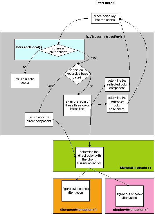
It's your choice to implenment shade() in class Material, or implement everything you need in class RayTracer
Before you try to code up a solution for the color model, be sure that you have a pretty good idea of how to do it on paper. Some of the vector math can start to look pretty overwhelming if you don't know what you are doing. Even when you do know what you are doing, there can be some rather tricky pitfalls... Three different things contribute to the color of a certain object:
| Direct Component | This component is calculated using the Blinn-Phong shading model. In general, you should iterate over every light in the scene and sum their individual contributions to the color intensity. There are some further complications here, because you have to deal with two different kinds of light sources when you are performing the computation: point lights and directional lights. Point lights have only position, and they radiate light outwards in all directions. Directional light only has a direction to it, and no starting position. Point light sources are better for modeling things such as light bulbs, while directional light is better for modeling something like sunshine. The two functions are worth noting because you need to implement the distance and shadow attenuation for each light in order for the Blinn-Phong shading model to work correctly. |
| Reflected Component | In order to calculate this component, you will need to calculate the reflection vector, and then make a recursive call to the traceRay function. |
| Refracted Component | Like the reflective component, this also needs to make recursive calls to the traceRay function. In addition, you also need to do some tests for total internal refraction, and handle this case accordingly. |
Because ray/object intersections are typically the bottleneck of ray tracing programs, the skeleton code uses a few techniques to try to speed it up. If an object's position is described by a transformation M, then M inverse is applied to both the object and the ray. This transforms the object back to the origin, which simplifies intersection testing.
For each object, the intersection testing occurs in the object's IntersectLocal function. By the time control has been given to this function, the object and ray have already been translated back to the origin, so you don't have to worry about doing that. Additionally, you don't have to worry about translating the object and ray back to their original position; this is done after the function exits. You only have to worry about the intersection of the input ray and the basic, untransformed object (i.e., untransformed spheres are centered at the origin with a radius of one). We also provide the constant RAY_EPSILON for your use. If an intersection is then found, some information about the object needs to be calculated. The Normal and t-value for the intersection need to be properly set, so that the information can later be used to calculate lighting information. All of this information should be stored in the Intersection "i" argument that is passed by reference into IntersectLocal. Intersection is described in scene/ray.h.
Once you implement the requirements, you'll be able to verify your implemetation. We provide several sample scenes you can use to compare your ray tracer to the solution with in assets/trace. Start with the scenes in the simple/ directory, which will help isolate any bugs or odd behavior you may find.
We also provide automate diff tool for you, to compare your traing result with the sample solution. There are two ways you may use the tool:
You can also use an image diff tool such as the one here to compare images.
Don't worry if your solution doesn't give exactly the same output (rounding errors, among other things, are a fact of life). However, if there is a noticeable pattern in the errors, then that definitely means something is wrong! This tool is only to get an idea of where to look for problems. Note that your bells and whistles must be disabled for the tool to accurately check against the sample.
Memory Leaks: It is strongly advised your program does not have any memory leaks! For more information check out this summary. To check if you have a memory leak in ray.exe, render dragon full depth, antialiasing, max size, etc. on Windows, do a ctrl+shift+Esc and watch ray.exe's memory consumption. If it is increasing to no end you probably have a leak. It is likely the program will crash out after some point. Why do we care?! It is extremely frustrating for your render to stop at "91% complete" on the night of Artifact turn in!
As you get into the project, you'll probably want to make your own scenes (besides the ones in assets/trace) using the modeling features of the software. To create realistic refractive objects, you'll need their Indices of Refraction.
The Qt codebase contains code to parse triangular mesh models saved in standard .ply format.
Here are step-by-step instructions for importing models using Blender, a heavier weight tool for 3D models. You can do a lot more with it. Please feel free to explore its potentials.
Open up Blender and clear the scene. To do this, hit "A" until all objects (including the camera and viewer) are selected (they'll turn orange), then delete by pressing Delete then Enter.
Load your model file via File->Import. You'll want to make sure that it's all one mesh; occasionally 3D models come as a collection of different pieces which are each individual meshes. Hit A until everything is selected, then press CTRL-J to join all of the objects into a single mesh.
We'll need to edit the mesh a bit, since sometimes meshes contain quads and we want to convert them to trianlges.
Go to the mode selection (it should say "Object Mode" by default, near the bottom of the screen) and select "Edit Mode." You should see all of the faces in your model selected; if not, hit A until they're all selected. Hit CTRL-F to bring up the Faces menu. Select "Triangulate Faces" to convert them all into trianlges. Now press CTRL-F again, and select "Shade Smooth" (I'm pretty sure this ensures that your vertices all have per-vertex normals).
Now you're ready to export. If you want to edit material properties or play with the geometry before doing so, feel free.
With the object still selected, go to "File->Export->Stanford (.ply)". Pick a directory and filename for your output file. Hit "Export PLY" to export the file.
Then you can import that .ply file into your program as a mesh, create that mesh, set up your lights and a render camera, and render the scene!
Please follow the general instructions here. More details below:
Each team is required to submit one artifact per person. Name the file [your-cse-netid].jpg or [your-cse-netid].png. The scene traced cannot be one of the provided .yaml files but must at least be modified in some way (or a completely new scene). With each artifact, you may also submit some brief comments -- this can be as simple as two sentences describing the placement of the objects and lights to get the desired effect or a detailed description of the bells and whistles used to create the scene. The comments will be posted with your artifact on the webpage for voting.
Important: There is much room to create something really cool for your artifact, and we encourage you to spend a little time on it (at least more than 10 minutes!). In particular, your Trace artifact should not be too similar to one of the sample scenes. If your rendering is simply based on a tweaked version of a sample scene (e.g., you just rotated the camera X degrees in two axes, or changed the color of an object) then you will lose some (easy) points on turn in.
If you implement any bells or whistles you need to provide examples of these features in effect. You should present your extra credit features at grading time either by rendering scenes that demonstrate the features during the grading session or by showing images you rendered in advance. You might need to pre-render images if they take a while to compute (longer than 30 seconds). These pre-rendered examples, if needed, must be included in your turnin directory on the project due date. The scenes you use for demonstrating features can be different from what you end up submitting as an artifact.
Important: You need to establish to our satisfaction that you've implemented the extension. Create test cases that clearly demonstrate the effect of the code you've added to the ray tracer. Sometimes different extensions can interact, making it hard to tell how each contributed to the final image, so it's also helpful to add controls to selectively enable and disable your extensions. In fact, we require that all extensions be disabled by default, with controls to turn them on one by one.
Both Marschner and Shirley's book and Foley, et al., are reasonable resources for implementing bells and whistles. In addition, Glassner's book on ray tracing is a very comprehensive exposition of a whole bunch of ways ray tracing can be expanded or optimized (and it's really well written). If you're planning on implementing any of these bells and whistles, you are encouraged to read the relevant sections in these books as well.
Here are some examples of effects you can get with ray tracing. Currently, none of these were created from past students' ray tracers.
 |
Implement an adaptive termination criterion for tracing rays, based on ray contribution. Control the adaptation threshold with a slider or spinbox. |
 |
Modify your antialiasing to sample at random positions within a pixel. This is trades aliasing for noise, which the eye is less sensitive to, and used in Monte Carlo path tracing. The noise introduced by this random sampling should be evident when casting 1 ray per pixel. |
 |
Modify your antialiasing to jitter the sub-pixel samples, i.e., randomly sample positions within each sub-pixel region of a pixel (after breaking the pixel into a set of small squares). See Marschner Shirley 13.4.1. This is a form of stratified sampling to reduce noise in Monte Carlo path tracing. As with the previous whistle, the noise introduced by jittering should be evident when casting 1 ray per pixel. |
 |
Modify shadow attenuation to use Beer's Law, so that the thicker objects cast darker shadows than thinner ones with the same transparency constant. (See Marschner Shirley p. 325.) |
 |
Include a Fresnel term so that the amount of reflected and refracted light at a transparent surface depend on the angle of incidence and index of refraction. (See Marschner Shirley p. 325.) |
 |
Implement spotlights. You'll have to extend the parser to handle spot lights but don't worry, this is low-hanging fruit. |
 |
Improve your refraction code to allow rays to refract correctly through objects that are contained inside other objects. You must put together a .yaml file to demonstrate this effect. |
 |
Find a good way to accelerate shadow attenuation. Do you need to check against every object when casting the shadow ray? This one is hard to demonstrate directly, so be prepared to explain in detail how you pulled it off. |
 |
Deal with overlapping objects intelligently. While the skeleton code handles materials with arbitrary indices of refraction, it assumes that objects don't intersect one another. It breaks down when objects intersect or are wholly contained inside other objects. Add support to the refraction code for detecting this and handling it in a more realistic fashion. Note, however, that in the real world, objects can't coexist in the same place at the same time. You will have to make assumptions as to how to choose the index of refraction in the overlapping space. Make those assumptions clear when demonstrating the results. |
 |
Implement antialiasing by adaptive supersampling. For full credit, you must show some sort of visualization of the sampling pattern that results. For example, you could create another image where each pixel is given an intensity proportional to the number of rays used to calculate the color of the corresponding pixel in the ray traced image. Implementing this bell/whistle is a big win -- nice antialiasing at low cost. |
 x2 x2 |
Add a menu option that lets you specify a background images cube to replace the environment's ambient color during the rendering. That is, any ray that goes off into infinity behind the scene should return a color from the loaded image on the appropriate face of the cube, instead of just black. The background should appear as the backplane of the rendered image with suitable reflections and refractions to it. This is also called environment mapping. Click here for some examples and implementation details and here for some free cube maps (also called skyboxes). |
 x2 x2 |
|
 x2 x2 |
Implement solid textures or some other form of procedural texture mapping. Solid textures are a way to easily generate a semi-random texture like wood grain or marble. Click here for a brief look at making realistic looking marble using Ken Perlin's noise function. |
 x2 x2 |
Add some new types of geometry to the ray tracer. Consider implementing torii or general quadrics. Many other objects are possible here. |
 x2 x2 |
Extend the ray-tracer to create Single Image Random Dot Stereograms (SIRDS). Click here to read a paper on how to make them. Or, create 3D images like this one, for viewing with red-blue glasses. |
 x2* x2* |
Implement Monte Carlo path tracing to produce one or more or the following effects: depth of field, soft shadows, motion blur, or glossy reflection. For additional credit, you could implement stratified sampling (part of "distribution ray tracing") to reduce noise in the renderings. (See lecture slides, Marschner Shirley 13.4). *You will earn 2 bells for the first effect, and 2 whistles for each additional effect. |
 x2 x2 |
Implement a more realistic shading model. Credit will vary depending on the sophistication of the model. A simple model factors in the Fresnel term to compute the amount of light reflected and transmitted at a perfect dielectric (e.g., glass). A more complex model incorporates the notion of a microfacet distribution to broaden the specular highlight. Accounting for the color dependence in the Fresnel term permits a more metallic appearance. Even better, include anisotropic reflections for a plane with parallel grains or a sphere with grains that follow the lines of latitude or longitude. Sources: Shirley, Chapter 24, Watt, Chapter 7, Foley et al, Section 16.7; Glassner, Chapter 4, Section 4; Ward's SIGGRAPH '92 paper; Schlick's Eurographics Rendering Workshop '93 paper. This all sounds kind of complex, and the physics behind it is. But the coding doesn't have to be. It can be worthwhile to look up one of these alternate models, since they do a much better job at surface shading. Be sure to demo the results in a way that makes the value added clear. Theoretically, you could also invent new shading models. For instance, you could implement a less realistic model! Could you implement a shading model that produces something that looks like cel animation? Variable extra credit will be given for these "alternate" shading models.Note that you must still implement the Blinn-Phong model. |
 x3 x3 |
Add some higher-level geometry to the ray tracer, such as extrusions, metaballs, swept surfaces, or blend surfaces. You may have implemented one or more of these as a polygonal object in the modeler project. For the Raytracer, be sure you are actually raytracing the surface as a mathematical construct, not just creating a polygonal representation of the object and tracing that. Yes, this requires lots of complicated math, but the final results are definitely worth it (see Transparent Metaballs). Here is a really good tutorial on raytracing metaballs. For an additional bell, add texture mapping to your higher-level geometry. The texture mapping must look good in order to get credit for it! |
 x3 x3 |
Implement ray-intersection optimization by either significantly extending the BSP Tree implemented in the skeleton or by implementing a different optimization method, such as hierarchical bounding volumes (See Marschner Shirley 12.3). |
 x3 x3 |
Implement 3D fractals and extend the .yaml file format to provide support for these objects. Note that you are not allowed to "fake" this by just drawing a plain old 2D fractal image, such as the usual Mandelbrot Set. Similarly, you are not allowed to cheat by making a .yaml file that arranges objects in a fractal pattern. You must raytrace an actual 3D fractal, and your extension to the .yaml file format must allow you to control the resulting object in some interesting way, such as choosing different fractal algorithms or modifying the base pattern used to produce the fractal. Here are two really good examples of raytraced fractals that were produced by students during a previous quarter: Example 1, Example 2 And here are a couple more interesting fractal objects: Example 3, Example 4 |
 x4 x4 |
Implement 4D quaternion fractals and extend the .yaml file format to provide support for these objects. These types of fractals are generated by using a generalization of complex numbers called quaternions. What makes the fractal really interesting is that it is actually a 4D object. This is a problem because we can only perceive three spatial dimensions, not four. In order to render a 3D image on the computer screen, one must "slice" the 4D object with a three dimensional hyperplane. Then the points plotted on the screen are all the points that are in the intersection of the hyperplane and the fractal. Your extension to the .yaml file format must allow you to control the resulting object in some interesting way, such as choosing different generating equations, changing the slicing plane, or modifying the surface attributes of the fractal. Here are a few examples, which were created using the POV-Ray raytracer (yes, POV-Ray has quaternion fractals built in!): Example 1, Example 2, Example 3, Example 4. And, this is an excellent example from a previous quarter. To get started, visit this web page to brush up on your quaternion math. Then go to this site to learn about the theory behind these fractals. Then, you can take a look at this page for a discussion of how a raytracer can perform intersection calculations. |
 x4 x4 |
Implement CSG, constructive solid geometry. This extension allows you to create very interesting models. See page 108 of Glassner for some implementation suggestions. An excellent example of CSG was built by a grad student here in the grad graphics course. |
 x4 x4 |
Implement caustics by tracing rays from the light source and depositing energy in texture maps (a.k.a., illumination maps, in this case). Caustics are variations in light intensity caused by refractive focusing--everything from simple magnifying-glass points to the shifting patterns on the bottom of a swimming pool. Here is a paper discussing some methods. 2 bells each for refractive and reflective caustics. (Note: caustics can be modeled without illumination maps by doing "photon mapping", a monster bell described below.) Here is a really good example of caustics that were produced by two students during a previous quarter: Example |
There are innumerable ways to extend a ray tracer. Think about all the visual phenomena in the real world. The look and shape of cloth. The texture of hair. The look of frost on a window. Dappled sunlight seen through the leaves of a tree. Fire. Rain. The look of things underwater. Prisms. Do you have an idea of how to simulate this phenomenon? Better yet, how can you fake it but get something that looks just as good? You are encouraged to dream up other features you'd like to add to the base ray tracer. Obviously, any such extensions will receive variable extra credit depending on merit (that is, coolness!). Feel free to discuss ideas with the course staff before (and while) proceeding!
Disclaimer: please consult the course staff before spending any serious time on these. These are all quite difficult (I would say monstrous) and may qualify as impossible to finish in the given time. But they're cool.
 |
Sub-Surface ScatteringThe trace program assigns colors to pixels by simulating a ray of light that travels, hits a surface, and then leaves the surface at the same position. This is good when it comes to modeling a material that is metallic or mirror-like, but fails for translucent materials, or materials where light is scattered beneath the surface (such as skin, milk, plants... ). Check this paper out to learn more. |
 |
Metropolis Light TransportNot all rays are created equal. Some light rays contribute more to the image than others, depending on what they reflect off of or pass through on the route to the eye. Ideally, we'd like to trace the rays that have the largest effect on the image, and ignore the others. The problem is: how do you know which rays contribute most? Metropolis light transport solves this problem by randomly searching for "good" rays. Once those rays are found, they are mutated to produce others that are similar in the hope that they will also be good. The approach uses statistical sampling techniques to make this work. Here's some information on it, and a neat picture. |
 |
Photon MappingPhoton mapping is a powerful variation of ray tracing that adds speed, accuracy and versatility. It's a two-pass method: in the first pass photon maps are created by emitting packets of energy photons from the light sources and storing these as they hit surfaces within the scene. The scene is then rendered using a distribution ray tracing algorithm optimized by using the information in the photon maps. It produces some amazing pictures. Here's some information on it. Also, if you want to implement photon mapping, we suggest you look at the SIGGRAPH 2004 course 20 notes (accessible from any UW machine or off-campus through the UW library proxy server). |