|

Project 4 : Animator
Assigned: 5/21
Due : Tuesday, 6/3, 11:59pm
Snapshot Due : Tuesday, 6/3, 11:59pm
Artifact Due : Wednesday, 6/4, 9:00am
Help sessions (Sieg 327):
#1: Tuesday, May 27th at 5:00pm
#2: Wednesday, May 28th at 5:00pm
Project TA : Joshua Barr & Chris Gonterman
|
Quick Links
- Skeleton Code
- Sample Solution
- FLTK
Libraries 1.1.7
- Configuring FLTK at Home
- Fluid executable
- Witkin's
and Baraff's Physically Based Modeling: Differential Equations Basics
- Witkin's Physically Based
Modeling: Particle System Dynamics
- Pseudocode for connecting
Particle Systems to hierarchies
- John Lasseter's article on Animation
Principles
- C2 interpolating curve notes (look
at pages 13 and 14) by Bartels, Beatty, and Barsky
- Demos:
- Autumn 07
Help Session (with video
clips)
- Putting together your final artifact
- Inspiring projects from previous quarters
Project Objectives
In this project, you are required to extend a spline-based animation system
to support multiple curve types, and implement a particle system simulation engine.
After building a working system, you will use your (robust and powerful)
program to produce a (compelling and arresting) animation.
Overview
The skeleton code provided is built on top of the same architecture as the Modeler,
and is designed so that you can re-use your models. If you replace robotarm.cpp
with a working model file from Project 2, you should be able to compile the
program and play with the interface. As with the Modeler, this
application has two windows: a viewer for the model, and a main window that
allows you to manipulate the various model and camera parameters. If you
click on the "Controls" tab in the main window, you will essentially
get the Modeler interface, with sliders for controlling components of
your character. The second mode, where you'll be spending most of your
time, is the "Curves" mode. Curves mode is where you edit a
time-varying curve for each model parameter by adding and moving control
points. Selecting controls in the left-hand browser window brings up the
corresponding curves in the graph on the right. Here, time is plotted on
the x-axis, and the value of a given parameter is plotted on the y-axis.
This graph display and interface is encapsulated in the GraphWidget
class.
Project Requirements
Here is a summary
of the requirements for this project:
- Implement
the following curve types:
- Bezier
(cubic beziers
splined together with C0 continuity)
- Catmull-Rom
(with endpoint interpolation)
- B-spline
(with endpoint interpolation)
- Implement
a particle system that:
- is
attached to a node of your hierarchy other than the root node.
- has
two distinct forces acting on the particles.
- includes
collision detection and response and provide control of the restitution
constant.
FLUID
In the skeleton code distribution, we've included the fluid file for the AnimatorUIWindows
class (animatoruiwindows.fl). In addition, we've included the
binary for fluid so that you can
make additions to the UI if you want.
Graph Widget Interface
After selecting a series of model parameters in the browser window, their
corresponding animation curves are displayed in the graph. Each spline is
evaluated as a simple piece-wise linear curve that linearly interpolates
between control points. You can manipulate the curves as follows:
|
Command |
Action |
| LEFT MOUSE |
Clicking anywhere in the graph creates a control point for
the selected curve. Control points can be moved by clicking on them and dragging. |
| CTRL LEFT MOUSE |
Selects the curve |
| SHIFT LEFT MOUSE |
Removes a control point |
| ALT LEFT MOUSE |
Rubber-band selection of control points |
| RIGHT MOUSE |
Zooms in X and Y dimensions |
| CTRL RIGHT MOUSE |
Zooms into the rubber-banded space region |
| SHIFT RIGHT MOUSE |
Pans the viewed region |
Note that each of the displayed curves has a
different scale. Based on the maximum and minimum values for each
parameter that you specified in your model file, the curve is drawn to
"fit" into the graph. You'll also notice that the other curve types
in the drop-down menu are not working. One part of your requirements (outlined
below) is to implement these other curves.
Controlling Time
At the bottom of the window is a simple set of VCR-style controls and a time
slider that let you play, pause, and seek in your animation. The Loop button will make the animation start over
when it reaches the end. The Simulate button relates to the
particle system which is discussed below.
Controlling the Camera
Camera motions can be edited in two ways:
- Setting
Keyframes: You will use the camera keyframing interface to define
some basic camera movements. The Set button will take the
current camera parameters from the viewport and save them as control points
in the graph widget. Typically, you will move the time slider,
adjust the camera pose in the viewport, then click Set. If
you want to remove a keyframe, use the time slider to seek to the
approximate time of the keyframe, then click "Remove" button.
Remove will delete all camera control points in a narrow range around the
current time.
- Editing
Curves: There are 8 camera parameters that appear as the last 8
items in the Model Controls list. Clicking on one of these
properties will cause the control points for this curve to appear in the
graph widget interface. From here, you can edit control points and
curve types as you can with any other model parameter.
Animation Curves
The GraphWidget object owns a bunch of Curve objects. The Curve
class is used to represent the time-varying splines associated with your model
parameters. You don't need to worry about most of the existing code,
which is used to handle the user interface. However, it is important that
you understand the curve evaluation model. Each curve is represented by a
vector of evaluated points.
mutable std::vector
    m_ptvCtrlPts;

    mutable std::vector m_ptvEvaluatedCurvePts;
The user of your program can manipulate the positions of the control points
using the Graph Widget interface. Your code will compute the value of
the curve at intervals in time, determining the shape of the curve. Given a set
of control points, the system figures out what the evaluated points are.
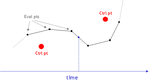
This conversion process is handled by the CurveEvaluator member
variable of each curve.
const CurveEvaluator* m_pceEvaluator;
In the skeleton, only the LinearCurveEvaluator has been implemented. Consequently,
the curve drawn is composed of line segments directly connecting each control
point. You should use the LinearCurveEvaluator as a model to
implement the other required curve evaluators: Bezier, B-Spline, and
Catmull-Rom. C2-Interpolating curves can be added for extra
credit.
Adding Curve Types
For each curve type, you must write a new class that inherits from CurveEvaluator.
Inside the class, you should implement the evaluateCurve function. This
function takes the following parameters:
ptvCtrlPts--a collection of control
points that you specify in the curve editor
ptvEvaluatedCurvePts--a
collection of evaluated curve points that you return from the function
calculated using the curve type's formulas
fAniLength--the maximum time
that a curve is defined
bWrap--a flag indicating
whether or not the curve should be wrapped (wrapping can be implemented for
extra credit)
To add a new curve
type, you should look in the GraphWidget constructor and change the
following lines to use your new set of evaluator classes.
m_ppceCurveEvaluators[CURVE_TYPE_BSPLINE]
= new LinearCurveEvaluator();
m_ppceCurveEvaluators[CURVE_TYPE_BEZIER] = new LinearCurveEvaluator();
m_ppceCurveEvaluators[CURVE_TYPE_CATMULLROM] = new LinearCurveEvaluator();
For Bezier curves (and the splines based on them), it is sufficient to
sample the curve at fixed intervals of time. The adaptive de Casteljau
subdivision algorithm presented in class may be implemented for an extra bell.
Catmull-Rom and B-spline curves should be endpoint interpolating. This can
be done by doubling the endpoints for Catmull-Rom and tripling them for
B-spline curves.
You do not have to sort the control points or the evaluated curve points.
This has been done for you. Note, however, that for an interpolating curve
(Catmull-Rom), the fact that the control points are given to you sorted by x
does not ensure that the curve itself will also monotonically increase in x.
You should recognize and handle this case appropriately. One solution is
to return only the evaluated points that are increasing monotonically in x.
Also, be aware that the evaluation function will linearly interpolate
between the evaluated points to ensure a continuous curve on the screen.
This is why you don't have to generate infinitely many evaluated points.
Particle System Simulation
The skeleton code has a very high-level framework in place for running
particle simulations that is based on Witkin's Particle System
Dynamics. In this model, there are three major components:
- Particle
objects (which have physical properties such as mass, position and
velocity)
- Forces
- An
engine for simulating the effect of the forces acting on the particles
that solves for the position and velocity of each particle at every time
step
You are responsible for coming up with a representation for particles and
forces. The skeleton provides a very basic outline of a simulation
engine, encapsulated by the ParticleSystem class. Currently, the
header file (ParticleSystem.h) specifies an interface that must
be supported in order for your particle system to interact correctly with the
animator UI. Alternately, you can try to figure out how the UI works
yourself by searching within the project files for all calls to the particle
system's functions, and then re-organizing the code. This second option
may provide you with more flexibility in doing some very ambitious particle
systems with extra UI support. However, the framework seems general enough
to support a wide range of particle systems. There is detailed
documentation in the header file itself that indicates what each function you
are required to write should do. Note that the ParticleSystem
declaration is by no means complete. As mentioned above, you will have to
figure out how you want to store and organize particles and forces, and as a
result, you will need to add member variables and functions.
One of the functions you are required to implement is called computeForcesAndUpdateParticles:
virtual void computeForcesAndUpdateParticles(float
t);
This function represents the meat of the simulation solver. Here you
will compute the forces acting on each particle and update their positions and
velocities based on these forces using Euler's method. As mentioned
above, you are responsible for modeling particles and forces in some way that
allows you to perform this update step at each frame.
Particles As Part of a Hierarchy
One requirement of your particle system is to attach it to a node of your
model other than the root. This requires that you think carefully about
about how to represent the positions of your particles.
Suppose you want to attach a particle shower to your model's hand.
When you apply the force of gravity to these particles, the direction of the
force will always be along the negative Y axis of the world. If you
mistakenly apply gravity along negative Y of the hand's coordinate space,
you'll see some funky gravity that depends on the orientation of the hand
(bad!). To solve this problem, we recommend that you attach a particle
emitter to the model's hand, but store all the particles positions as
coordinates in world space. This means that you'll need to calculate the
world coordinates of the particle emitter every time a particle is spawned.
Please read the following pseudocode,
which contains an in-depth discussion of using particles in your hierarchy.
The function getModelViewMatrix
is used in the file above. We are also providing the C implementation for
it:
Mat4f getModelViewMatrix()
{
GLfloat m[16];
glGetFloatv(GL_MODELVIEW_MATRIX, m);
Mat4f matMV(m[0], m[1], m[2], m[3],
m[4], m[5], m[6], m[7],
m[8], m[9], m[10], m[11],
m[12], m[13], m[14], m[15] );
    return matMV.transpose(); // because the matrix GL
returns is column major
}
Hooking Up Your Particle System
In the sample robotarm.cpp file, there is a comment in the main
function that indicates where you should create your particle system and hook
it up into the animator interface. After creating your ParticleSystem object,
you should do the following:
ParticleSystem *ps = new ParticleSystem();
...
// do some more particle system setup
...
ModelerApplication::Instance()->SetParticleSystem(ps);
Particle System Requirements
Here are the specific requirements for the particle system:
- Create
a particle system that is attached to a node of your model hierarchy other
than the root node.
- Implement
the simulation solver using Euler's method.
- Create
at least two distinct types of forces that act on your particle
system. The three most obvious distinct forces are gravity (f=mg),
viscous drag (f=-k_d*v), and Hooks spring law. Other interesting
possibilities include electromagnetic force, simulation of flocking
behavior, and buoyant force. If the forces you choose are complicated or
novel (or listed in the Bells and Whistles) you may earn extra credit
while simultaneously fulfilling this requirement.
- Perform
collision detection with your particles and at least one primitive in your
scene. A natural choice is the ground plane of your scene.
Your particles should bounce off of that primitive, and you should provide
a control for the restitution constant that determines how much the normal
component of the reflected velocity is attenuated.
- Hook
your particle system up to the application (See robotarm.cpp as an
example).
Once you've completed these tasks, you should be able to run your particle
system simulation by playing your animation with the Simulate button
turned on.
Animation Artifact
You will eventually use your program to produce an animated artifact for
this project (after the project due
date – see the top of the page for artifact due date). Under the File
menu of the program, there is a Save Movie As option, that will let you
specify a base filename for a set of movie frames. Each frame is saved as
a png or jpg. Use a program like Adobe Premiere (installed in the labs) to compress the
frame into a video file. (See Quick Links for more detail.)
Each group should turn in their own artifact. We may give extra credit to those
that are exceptionally clever or aesthetically pleasing. Try to use the ideas
discussed in the John Lasseter article.
These include anticipation, follow-through, squash and stretch, and secondary
motion.
Finally, plan for your animation to be 30 seconds long (60 seconds is the
absolute maximum). You will find this is a very small amount of time, so
consider this when planning your animation. We reserve the right to
penalize artifacts that go over the time limit and/or clip the video for the
purposes of voting. Refer to this guide for
creating your final .avi file.
- Absolute
time limit: 60 seconds...shorter is better!
- Animation
will count toward final grade on animator project.
- The
course staff will grade based on technical and artistic merit.
Voting:
- In-class
voting on Wednesday, June 4th, 2008
Bells and Whistles
![[whistle]](img/whistle.gif) Enhance the
required spline options. Some of these will require alterations to the user
interface, which involves learning Fluid and the UI framework. If you
want to access mouse events in the graph window, look at the handle
function in the GraphWidget class. Also, look at the Curve
class to see what control point manipulation functions are already
provided. These could be helpful, and will likely give you a better
understanding of how to modify or extend your program's behavior. A
maximum of 3 whistles will be given out in this category.
Enhance the
required spline options. Some of these will require alterations to the user
interface, which involves learning Fluid and the UI framework. If you
want to access mouse events in the graph window, look at the handle
function in the GraphWidget class. Also, look at the Curve
class to see what control point manipulation functions are already
provided. These could be helpful, and will likely give you a better
understanding of how to modify or extend your program's behavior. A
maximum of 3 whistles will be given out in this category.
- Let
the user control the tension of the Catmull-Rom spline
- Implement
one of the standard subdivision curves (e.g., Lane-Riesenfeld or
Dyn-Levin-Gregory).
- Add
options to the user interface to enforce C1 or C2
continuity between adjacent Bezier curve segments automatically. (It
should also be possible to override this feature in cases where you don't
want this type of continuity.)
- Add
the ability to add a new control point to any curve type without changing
the curve at all.
The linear curve
code provided in the skeleton can be "wrapped," which means that the
curve has C0 continuity between the end of the animation and the beginning. As
a result, looping the animation does not result in abrupt jumps. You will be
given a whistle for each (nonlinear) curve that you wrap.
Render a mirror in
your scene. As you may already know, OpenGL has no built-in reflection
capabilities. You can simulate a mirror with the following steps: 1) Reflect
the world about the mirror's plane, 2) Draw the reflected world, 3) Pop the
reflection about the mirror plane from your matrix stack, 4) Draw your world as
normal. After completing these steps, you may discover that some of the
reflected geometry appears outside the surface of the mirror. For an
extra whistle you can clip the reflected image to the mirror's surface, you
need to use something called the stencil buffer. The stencil buffer is
similar to a Z buffer and is used to restrict drawing to certain portions of
the screen. See Scott Schaefer's
site for more information. In addition, the NeHe game development site has
a detailed tutorial
Modify your
particle system so that the particles' velocities gets initialized with the
velocity of the hierarchy component from which they are emitted. The particles
may still have their own inherent initial velocity. For example, if your model
is a helicopter with a cannon launching packages out if it, each package's
velocity will need to be initialized to the sum of the helicopter's velocity
and the velocity imparted by the cannon.
Particles rendered
as points or spheres may not look that realistic. You can achieve more
spectacular effects with a simple technique called billboarding. A
billboarded quad (aka "sprite") is a textured square that always
faces the camera. See the
sprites demo. For full credit, you should load a texture with
transparency (sample textures), and
turn on alpha blending (see this tutorial
for more information). Hint: When rotating your particles to face the
camera, it's helpful to know the camera's up and right vectors in
world-coordinates.
Use the
billboarded quads you implemented above to render the following effects.
Each of these effects is worth one whistle provided you have put in a whistle
worth of effort making the effect look good.
- Fire (example) (You'll probably want to use
additive blending for your particles -
glBlendFunc(GL_SRC_ALPHA,GL_ONE);)
- Snow (example)
- Water
fountain (example)
- Fireworks
(example)
Use environment
mapping to simulate a reflective material. This technique is particularly
effective at faking a metallic material or reflective, rippling water
surface. Note that OpenGL provides some very useful functions for
generating texture coordinates for spherical environment mapping. Part of
the challenge of this whistle is to find these functions and understand how
they work.
Add baking to your
particle system. For simulations that are expensive to process, some
systems allow you to cache the results of a simulation. This is called
"baking." After simulating once, the cached simulation can then
be played back without having to recompute the particle properties at each time
step. See this page for more information on how
to implement particle baking.
Implement a motion
blur effect (example). The easy
way to implement motion blur is using an accumulation
buffer - however, consumer grade graphics cards do not implement an
accumulation buffer. You'll need to simulate an accumulation buffer by
rendering individual frames to a texture, then combining those textures.
See this
tutorial for an example of rendering to a texture.
Euler's method is
a very simple technique for solving the system of differential equations that
defines particle motion. However, more powerful methods can be used to
get better, more accurate results. Implement your simulation engine using
a higher-order method such as the Runge-Kutta technique. ( Numerical Recipes,
Sections 16.0, 16.1) has a description of Runge-Kutta and pseudo-code.
![[bell]](img/bell.gif) Implement
adaptive Bezier curve generation: Use a recursive, divide-and-conquer, de
Casteljau algorithm to produce Bézier curves, rather than just sampling
them at some arbitrary interval. You are required to provide some way to change
the flatness parameter and maximum recursion depth, with a keystroke or mouse
click. In addition, you should have some way of showing (a printf
statement is fine) the number of points generated for a curve to demonstrate
your adaptive algorithm at work.
Implement
adaptive Bezier curve generation: Use a recursive, divide-and-conquer, de
Casteljau algorithm to produce Bézier curves, rather than just sampling
them at some arbitrary interval. You are required to provide some way to change
the flatness parameter and maximum recursion depth, with a keystroke or mouse
click. In addition, you should have some way of showing (a printf
statement is fine) the number of points generated for a curve to demonstrate
your adaptive algorithm at work.
To get an extra whistle, provide visual controls in the UI (i.e. sliders) to
modify the flatness parameter and maximum recursion depth, and also display the
number of points generated for each curve in the UI.
Extend the particle
system to handle springs. For example, a pony tail can be simulated with a
simple spring system where one spring endpoint is attached to the character's
head, while the others are floating in space. In the case of springs, the
force acting on the particle is calculated at every step, and it depends on the
distance between the two endpoints. For one more bell, implement
spring-based cloth. For 2 more bells, implement spring-based fur.
The fur must respond to collisions with other geometry and interact with at
least two forces like wind and gravity.
Allow for particles
to bounce off each other by detecting collisions when updating their positions
and velocities. Although it is difficult to make this very robust, your
system should behave reasonably.
Implement a
"general" subdivision curve, so the user can specify an arbitrary
averaging mask You will receive still more credit if you can generate,
display, and apply the evaluation masks as well. There's a site at
Caltech with a few interesting applets that may be useful.
![[bell+whistle]](img/bell_whistle.gif) Add
a lens flare. This effect has components both in screen space and world
space effect.
For full credit, your lens flare should have at least 5 flare
"drops", and the transparency of the drops should change depending on
how far the light source is from the center of the screen. You do not
have to handle the case where the light source is occluded by other geometry
(but this is worth an extra whistle).
Add
a lens flare. This effect has components both in screen space and world
space effect.
For full credit, your lens flare should have at least 5 flare
"drops", and the transparency of the drops should change depending on
how far the light source is from the center of the screen. You do not
have to handle the case where the light source is occluded by other geometry
(but this is worth an extra whistle).
Perform
collision detection with more complicated shapes. For complex scenes, you
can even use the accelerated ray tracer and ray casting to determine if a
collision is going to occur. Credit will vary with the complexity shapes
and the sophistication of the scheme used for collision detection.
If
you find something you don't like about the interface, or something you think
you could do better, change it! Any really good changes will be
incorporated into the next Animator. Credit varies with the quality of
the improvement.
Add flocking
behaviors to your particles to simulate creatures moving in flocks, herds, or
schools. A convincing way of doing this is called "boids"
(see here for a demo and for more
information). For full credit, use a model for your creatures that makes
it easy to see their direction and orientation (for example, the yellow/green
pyramids in the boids demo would be a minimum requirement). For up to one
more bell, make realistic creature model and have it move realistically
according to its motion path. For example, a bird model would flap its
wings when it rises, and hold it's wings outstretched when turning.
Implement a C2-Interpolating
curve. There is already an entry for it in the drop-down menu.
Add the ability to
edit Catmull-Rom curves using the two "inner" Bezier control points
as "handles" on the interpolated "outer" Catmull-Rom
control points. After the user tugs on handles, the curve may no longer be
Catmull-Rom. In other words, the user is really drawing a C1
continuous curve that starts off with the Catmull-Rom choice for the inner
Bezier points, but can then be edited by selecting and editing the
handles. The user should be allowed to drag the interpolated point in a
manner that causes the inner Bezier points to be dragged along. See
PowerPoint and Illustrator pencil-drawn curves for an example.
Implement picking of
a part in the model hierarchy. In other words, make it so that you can
click on a part of your model to select its animation curve. To recognize
which body part you're picking, you need to first render all body parts into a
hidden buffer using only an emissive color that corresponds to an object
ID. After modifying the mouse-ing UI to know about your new picking mode,
you'll figure out which body part the user has picked by reading out the ID
from your object ID buffer at the location where the mouse clicked. This
should then trigger the GraphWidget to select the appropriate curve for
editing. If you're thinking of doing either of the inverse kinematics
(IK) extensions below, this kind of interface would be required.
If you implemented
twist for your original model, the camera movement for your old modeler can
give some unexpected results. For example, twist your model 90
degrees. Now try to do rotations as normal. This effect is called
gimbal lock. Change the camera to use quaternions as a method for
avoiding the gimbal lock.
Implement projected textures.
Projected textures are used to simulate things like a slide projector,
spotlight illumination, or casting shadows onto arbitrary geometry. Check
out this demo and read details
of the effect at glBase,
and SGI.
An alternative way to
do animations is to transform an already existing animation by way of motion
warping (animations).
Extend the animator to support this type of motion editing.
We've talked about
rigid-body simulations in class. Incorporate this functionality into your
program, so that you can correctly simulate collisions and response between
rigid objects in your scene. You should be able to specify a set of
objects in your model to be included in the simulation, and the user should
have the ability to enable and disable the simulation either using the existing
"Simulate" button, or with a new button.
Disclaimer: please consult the course staff before spending any
serious time on these. They are quite difficult, and credit can vary depending
on the quality of your method and implementation.

Inverse kinematics
The hierarchical model that you created is controlled by forward kinematics;
that is, the positions of the parts vary as a function of joint angles. More
mathematically stated, the positions of the joints are computed as a
function of the degrees of freedom (these DOFs are most often
rotations). The problem is inverse kinematics is to determine the DOFs of a
model to satisfy a set of positional constraints, subject to the DOF
constraints of the model (a knee on a human model, for instance, should not
bend backwards).
This is a significantly harder problem than forward kinematics. Aside from
the complicated math involved, many inverse kinematics problems do unique
solutions. Imagine a human model, with the feet constrained to the ground. Now
we wish to place the hand, say, about five feet off the ground. We need to
figure out the value of every joint angle in the body to achieve the desired
pose. Clearly, there are an infinite number of solutions. Which one is
"best"?
Now imagine that we wish to place the hand 15 feet off the ground. It's
fairly unlikely that a realistic human model can do this with its feet still
planted on the ground. But inverse kinematics must provide a good solution
anyway. How is a good solution defined?
Your solver should be fully general and not rely on your specific model
(although you can assume that the degrees of freedom are all rotational).
Additionally, you should modify your user interface to allow interactive
control of your model though the inverse kinematics solver. The solver should
run quickly enough to respond to mouse movement.
If you're interested in implementing this, you will probably want to consult
the CSE558
lecture notes.
Interactive Control of Physically-Based Animation
Create a character whose physics can be controlled by moving a mouse or
pressing keys on the keyboard. For example, moving the mouse up or down
may make the knees bend or extend the knees (so your character can jump), while
moving it the left or right could control the waist angle (so your character
can lean forward or backward). Rather than have these controls change
joint angles directly, as was done in the modeler project, the controls should
create torques on the joints so that the character moves in very realistic
ways. This monster bell requires components of the rigid body simulation
extension above, but you will receive credit for both extensions as long as
both are fully implemented.. For this extension, you will create a
hierarchical character composed of several rigid bodies. Next,
devise a way user interactively control your character.
This technique can produce some organic looking movements that are a lot of
fun to control. For example, you could create a little Luxo Jr. that hops
around and kicks a ball. Or, you could create a downhill skier that can
jump over gaps and perform backflips (see the Ski Stunt example below).
SIGGRAPH paper - http://www.dgp.toronto.edu/~jflaszlo/papers/sig2000.pdf
Several movie examples - http://www.dgp.toronto.edu/~jflaszlo/interactive-control.html
Ski Stunt - a fun game that implements this monster bell - Information and Java
applet demo - Complete Game (win32)
If you want, you can do it in 2D, like the examples shown in this paper (in
this case you will get full monster bell credit, but half credit for the rigid
body component).