Lecture 3 Summary
This was the first lecture at UW to use Tablet PCs for student
submissions. This might make the lecture easier to facilitate, since
the main points of interaction occurred around the classroom
activities. My feeling is that there was less verbal interaction in
this lecture than in the others. A description of the student
activities is given elsewhere.
I think that the usage of activities can follow the UW usage quite closely.
Lecture starts with an short discussion of the student submission
process - including enrouraging students to work together on
activities. I think we have been successful at the UW site of
establishing patterns of collaboration and participation. I want to
hear a lot of discussion when students are working on activities.

Activity One
The starting activity - draw something from Seattle was available at
the start of class - students had generally completed it before the
actual class happened. I would be happy to have the Beihang students
do this before class, since I am curious as to what their image of
Seattle is!


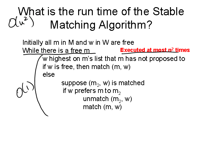
Run time discussion
At about 2 minutes a question is asked about what is the run time of
the Stable Matching algorithm, and what steps are necessary to allow
O(1) run time per update step.

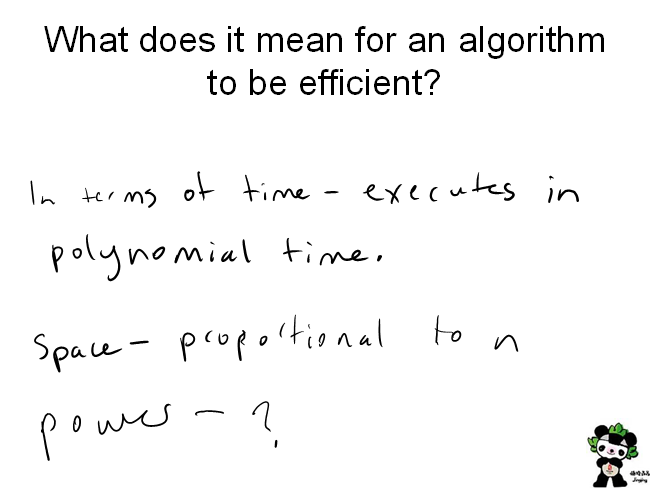
Activity Two
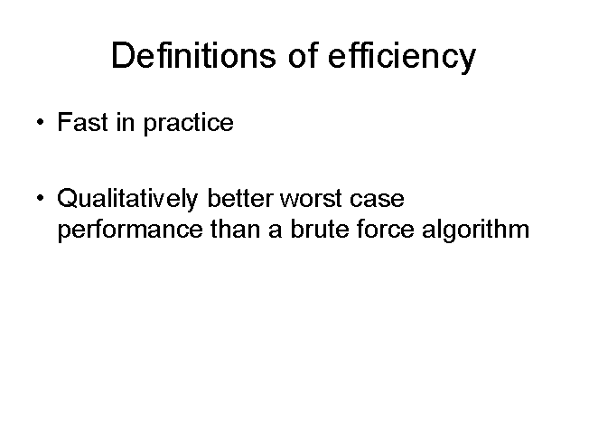
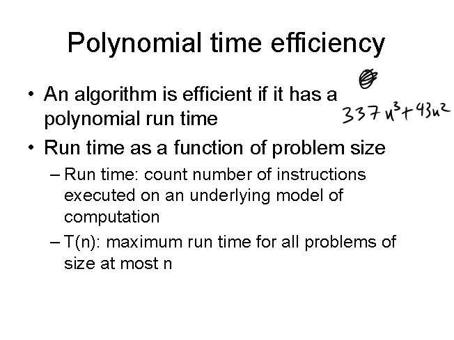
The second activity was to have the students provide a definition of
what it means for an algorithm to be efficient. I was hoping to use
the student definitions to distinguish between "theoretical"
definitions, and what it means to be "efficient in practice". The
answers didn't fall as neatly into these buckets. I think you should
use this activity as I did - and when you show the answers, try to
distinguish between the theoretical definitions, and the practical
definitions. I spent quite a bit of time discussing the answers to
this activity.
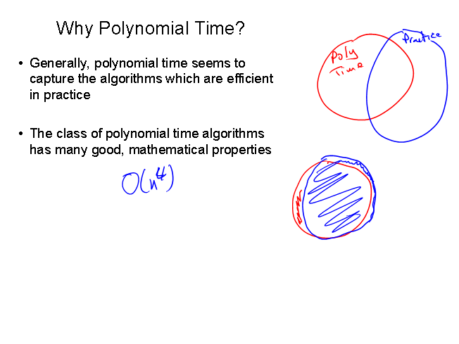
Polynomial time complexity
Slides 7-10, 13:24-21:28
This is a discussion of the reason why polynomial time complexity is a
useful notion. There are a a few quick questions that are asked to
the audience, that you may wish to get local answers to (although you
will need to be quick, since students answer at UW soon after the
question is posed).

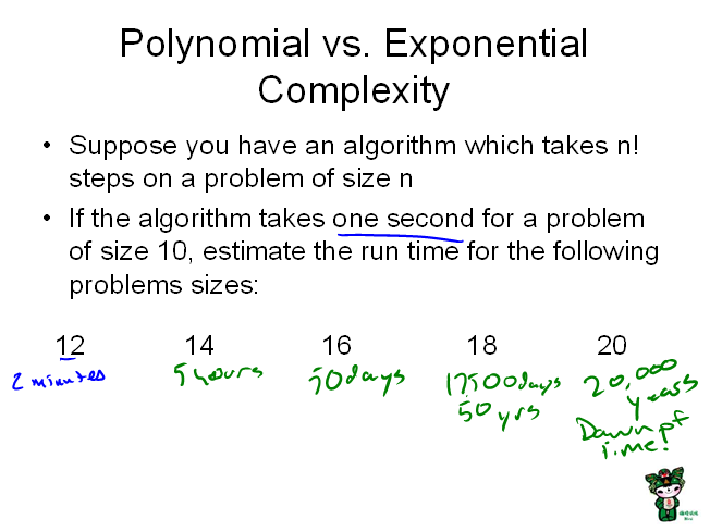
Activity Three: Factorial Complexity
This problem is to estimate the length of time to run an algorithm
with n! question. The key is to estimate the answers - not compute
them exactly. I don't want students using calculators for this. I
was actually confused by the answer when I discussed this in class -
and was off by a factor of 10 in the final column! (The activity
summary has the answer that I was looking for). I think this activity
is useful in that it does show how n! grows, and shows how impractical
it would be to solve a n! problem.

Ignoring constant factors

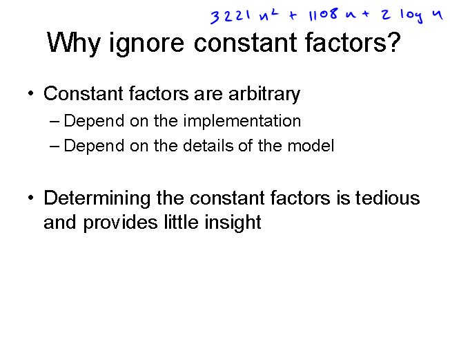

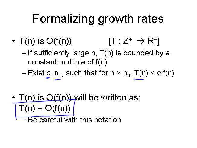
Activity Four
The activity is to do a big Oh proof by supplying the constants to
use. There are a wide range of constants that could work - so asking
students to provide the constants allowed them to participate in the
doing the proof.

