Lecture 2 Summary
This lecture was recorded with a very small audience - only four
people were present, two of them being students in the class, and the
other two were graduate students. There was also a technical problem
at the start of the lecture that required the first part of the
lecture to be repeated.
This lecture presented more advanced material on stable matchings.
The goal of the first lecture was to show a basic algorithm along with
its analysis and correctness proof. In contrast, the goal of the
second lecture is to show an advanced topic, and give the flavor of
the types of things that can be studied in an advanced course. There
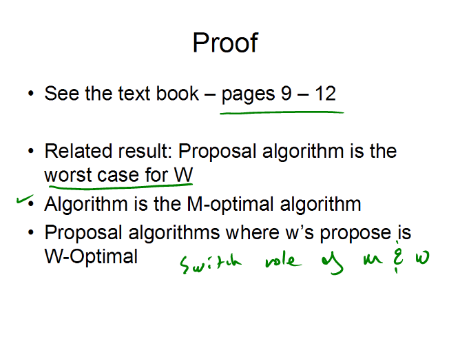
are two main results presented in this lecture. The first is that the
proposal algorithm is "Optimal" for the men, but worst case for the
women. The technical details of the proof are not presented - they
are in the text, and can be read by a motivated student. The second
result considers the average case analysis assuming that the
preference lists are random. This might give some insight into how
the algorithm would behave in practice. I think this is an
interesting result for the analysis of algorithms, and draws on some
probability theory. The result should be viewed strictly as
"enrichment" - if students don't understand the result, it will not
harm their performance later in the course. I hope that the result
will inspire some of the students to be more interested in the study
of algorithms.
In terms of spending time in class - more time should be spent on
lecture one, than on lecture two.
Introduction
Slide 1, 00:00-01:48
The initial question is raised - is the algorithm better for M's or
W's, this could be discussed.
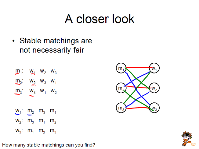
Example
Slide 3, 01:48-04:35
Have the students submit their answers, identifying the different
matchings. This is to show some matchings are good for the M's, and
some are good for the W's.
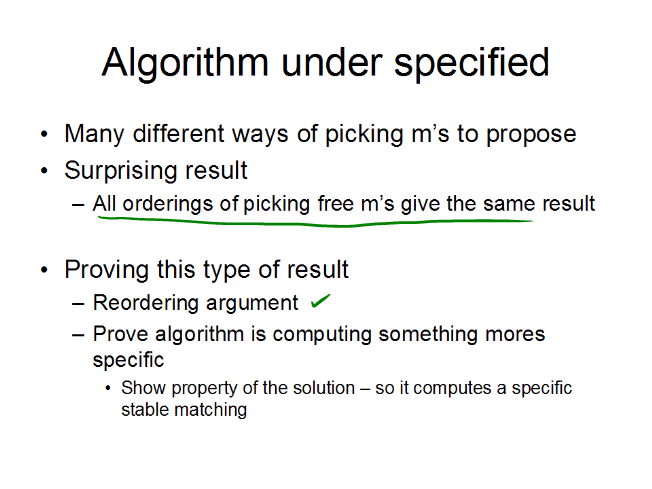
M-Optimal Theorem
Slides 4-6, 04:35-12:34
The main theorem is discussed. The goal of the discussion is to
provide a framework for someone to later read the proof in the text
book, and not to present the actual proof. There may not be much
discussion in this section.
A question is asked near the end of the discussion on slide six - how
to construct an optimal algorithm for W. You should stop the video
for this question.

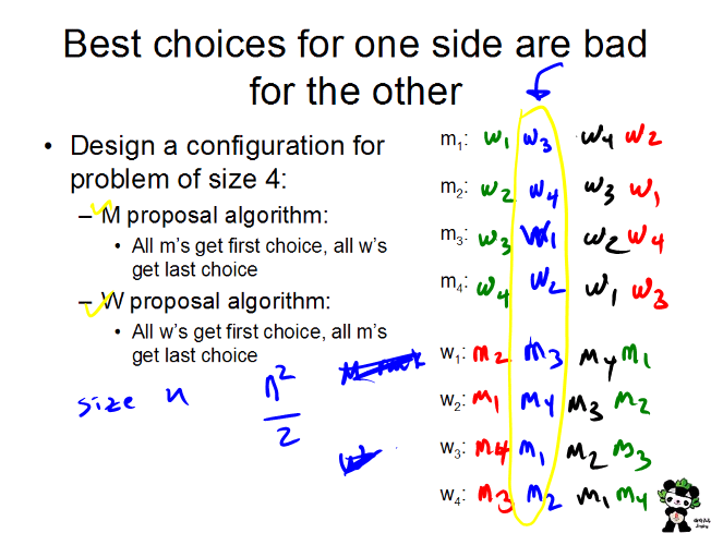
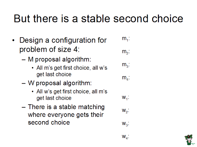
Example
Another example is generated which shows what is good for one side can
be bad for the other. This is done over a pair of slides, although in
class, it turned out easiest to use just a single slide.
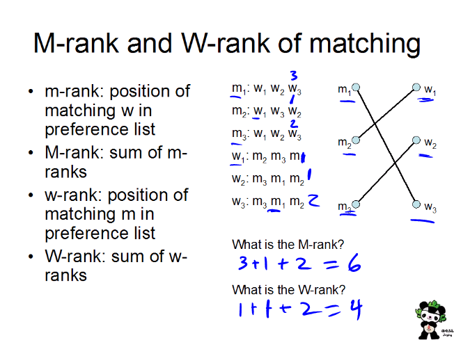
M-Rank, W-Rank
Following the summary slide, a pair of slides were used to define M-Rank. These can be done as
student submissions, and then discussed with the class.
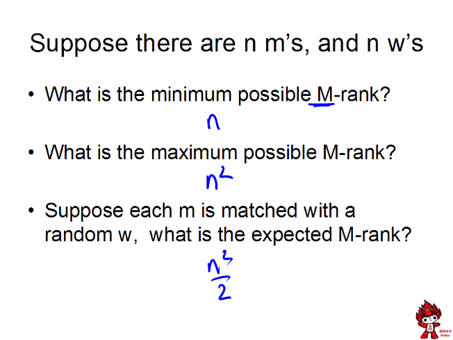
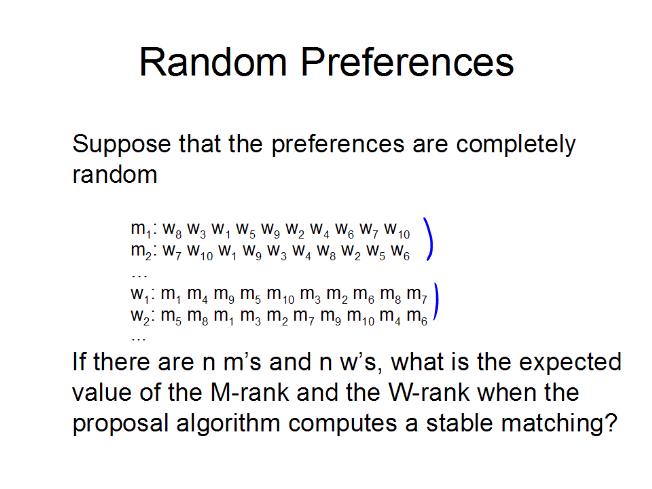
Average Case Analysis
Slides 12-16, 23:13-39:26
The question is now asked, what happens if the preferences lists are
random. The approach taken in class was to have students try to
predict what the M and W ranks would be. On the recorded version of
the class, it is hard to hear the student answer - which was that they
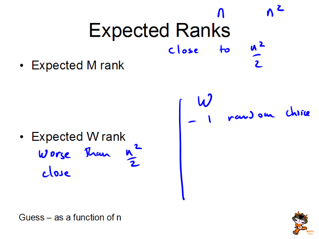
would both be close to n squared. This question is set up as a
student submission - but students might be hestitant to guess. You
could either do this as a student submission, or try to get students
to guess. However, if you can't get any student answers - just run
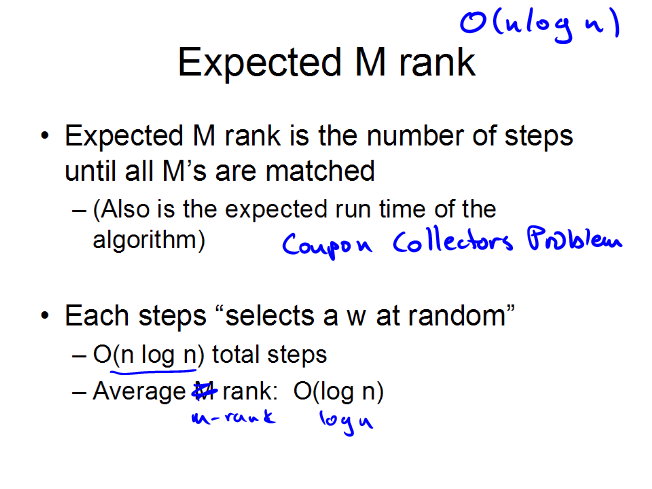
the lecture. The answer is that the M-rank is O(n log n), and the
W-rank is O(n2/log n), or to put it a different way, the
average m goes log n steps down his preference list, while the average
w is n/log n steps down her preference list.