Last week (and likely in CSE 373) you discussed Dijkstra’s algorithm for finding shortest paths in a graph. In our next class we will discuss a dynamic programming for finding shortest paths. In preparation for that, this reading addresses shortcomings of Dijkstra’s algorithm that our dynamic programming algorithm will overcome.

1 Review of Dijsktra’s algorithm

Let’s start by summarizing Dijkstra’s algorithm.

Input: a graph G and a start node s Output: a list of shortest path distances from s to every other node in the graph

shortestPath(G, s)
    set the priority[s] to 0, and the priority of all other nodes to infinity
    make a priority queue Q, add all nodes to it
    while Q is not empty:
        remove the lowest priority node x from Q
        for each neighbor y of x:
            if priority[y] > priority[x]+distance(x,y):
                priority[y] = priority[x]+distance(x,y)
                decrease priority of y in Q to match priority[y]
    return priority

The running time of this algorithm is then m \log(n) where m is the number of edges in the graph and n is the number of vertices. This is because:

• The outer while loop runs n times
• The number of times the inner for loop runs matches the out-degree of node y (i.e. the number of outgoing edges connected to y)
• Therefore the total cumulative number of iterations of the inner for loop matches the m, the number of edges in the graph (or 2m if the graph is undirected)
• each iteration of each loop does a constant number of priority queue operations that each cost \log(n) time to do

2 Key Assumption for Dijkstra’s Algorithm

For Disjkstra’s algorithm to correctly find shortest paths, we require that the graph has no negative-cost edges. If there are any edges with a negative weight then it is possible for Dijkstra’s algorithm to give us the wrong answer. Let’s look at an example.

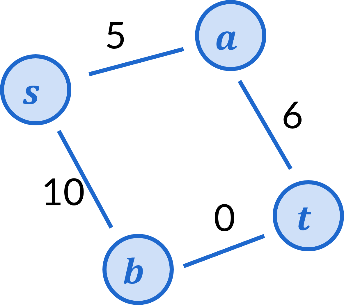
Consider the following graph:

Let’s step through what Dijksra’s algorithm does on this graph.

To begin, s has priority 0 and a,b,t all have priority \infty.

Next we remove s from the priority queue and assign priority 2 to a and 7 to b

Next we remove a from the priority queue and assign priority 5 to t.

Next we remove t from the priority queue, and this is where we get a problem.

We only update priorities for nodes that are still on the priority queue. Once a node has been removed, the algorithm will never consider any other paths to that node. In this case, therefore, the algorithm will discover the path s \rightarrow a \rightarrow t that has cost 5, and then never see the path s \rightarrow b \rightarrow t that has cost 4.

The intuitive reason that this happens is because Dijkstra’s algorithm visits nodes in the order of their currently-known distance from s. This is a perfectly find thing to do if edges all have non-negative weight, because that guarantees that once you’ve already accrued more cost to get from s to b compared to s to a there is no way to extend the s to b path to be lower-cost thn the s to a.

To put this is a different way, Dijkstra’s algorithm assumes that you cannot make a path lower-cost by include additional edges. Once we add in negative cost edges, though, this assumption no longer holds.

2.1 A Failed attempt at modifying Dijkstra’s

There are a few techniques you might consider for how to overcome Dijkstra’s limitation and compel the algorithm to work on negative-cost edges. We’re going to look at one such attempt and show that this doesn’t actually correct the problem.

The most common question I hear from students about Dijkstra’s algorithm is something like why can’t we just add a value to each edge’s weight so that none are negative. For example, the suggestion is to add 3 to the cost of every edge in the graph above to produce the following graph

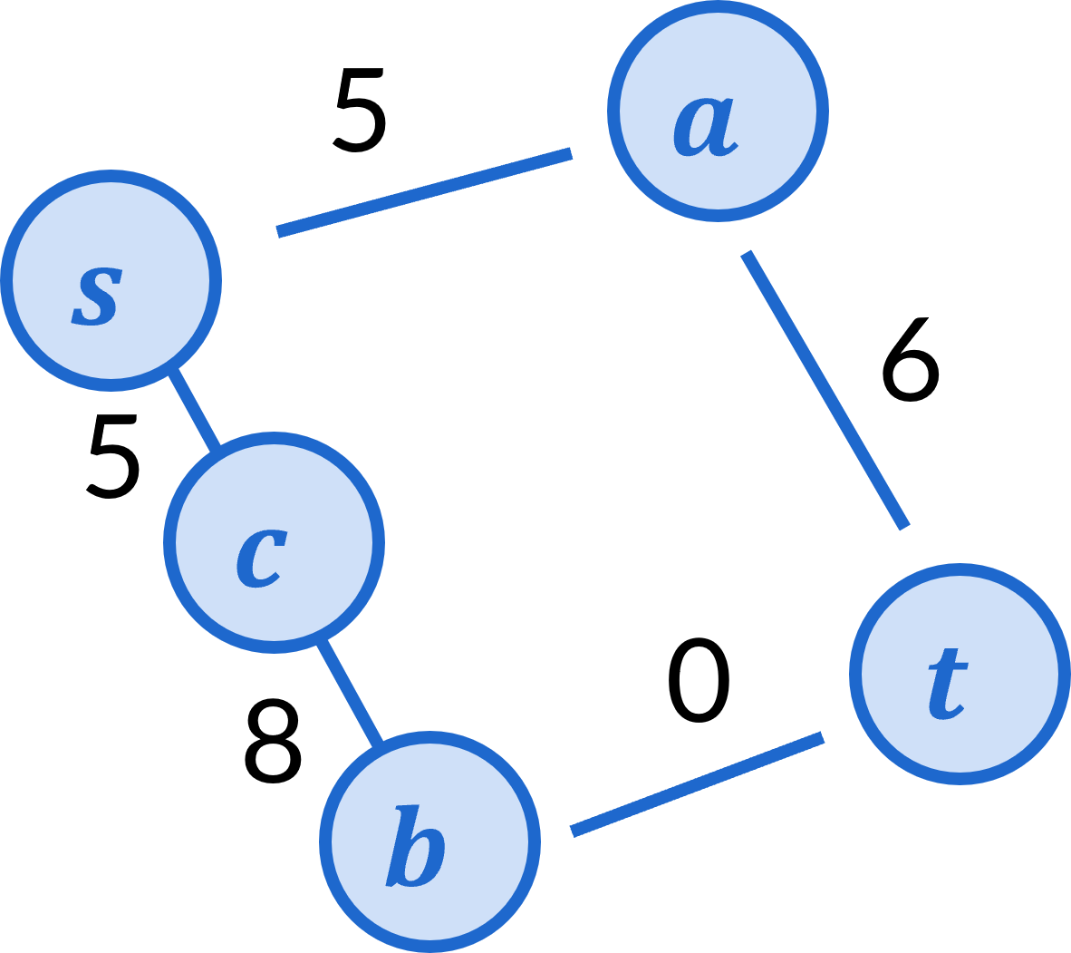
Running Dijkstra’s algorithm on this graph does correctly determine the least cost path from s to t is the s\rightarrow b \rightarrow t path. So it seems like a promising direction. But let’s consider this graph next. In this graph we split up the original graph’s edge of cost 7 to become two edges by inserting an intermediate node. One of the new edges has cost 2 and the other of cost 5.

For that graph, Dijkstra’s algorithm still incorrectly determines that the path s\rightarrow a \rightarrow t is the least cost. Now let’s see what our suggested strategy does to this graph. Again, we’re going to add 3 to each edge’s cost, giving the following graph as a result.

In this graph, Dijkstra’s algorithm still incorrectly determines that the path s\rightarrow a \rightarrow t is the least cost. The reason for this is because we are adding 3 to the cost of every edge, and so the amount a path’s cost increases depends on the number of edges along that path. The end result is that paths with more edges incurr more additional cost than paths with fewer edges.

It turns out that there is no known strategy for making a simple modification to Dijkstra’s algorithm to enable it to properly handle negative cost edges. We’ll need an entirely different algorithm for this. The algorithm we’ll discuss will leverage dynamic programming.

3 Negative cost cycles

There is one more major issue that we’ll need to address relating to negative cost edges. Weird things happen when we start considering shortest paths when there are negative cost cycles in the graph.

A cycle is defined as a path that starts and ends with the same node. For example, in our original path above, the path s\rightarrow a \rightarrow t \rightarrow b \rightarrow s is a cycle.

Let’s look a what happens when we consider shortest paths on the following graph.

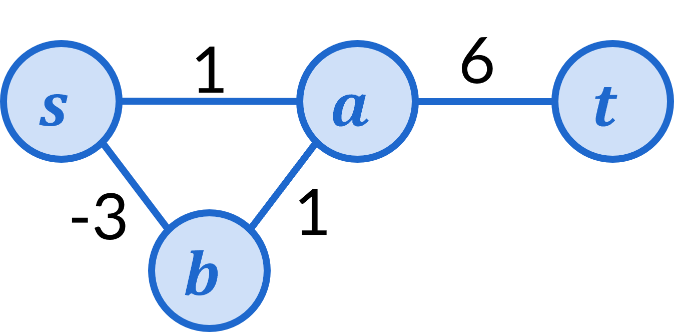
If we were to run Dijkstra’s algorithm to find the least cost path from s to t we would get the path s\rightarrow b \rightarrow a \rightarrow t which has cost 4. This might seem reasonable at first, however this is actually a better path than that! Because the cycle s\rightarrow b \rightarrow a \rightarrow s has cost -1, we could get a path of cost 3 by doing s\rightarrow b \rightarrow a \rightarrow s\rightarrow b \rightarrow a \rightarrow t. But why stop there?! We could get this cost down to 2 by taking the cycle twice! This would give the path s\rightarrow b \rightarrow a \rightarrow s\rightarrow b \rightarrow a \rightarrow s\rightarrow b \rightarrow a \rightarrow t. And we could keep doing this! Three spins of the cycle reduces the cost to 1, four spins reduces to to 0! In fact, we can never find a least cost path because we could always take the cycle more times to get a better path.

This all means that if a graph has negative cost cycles, a shortest path might not even exist!

4 Our next algorithm

This discussion motivates the details of what our next algorithm will need to do. Overall, we want an algorithm that finds shortest paths. To do this well, however, we also need to design the algorithm in a way where it is prepared for the fact that a shortest path might not exist. For this reason, our algorithm will do the following:

Input: a graph G and a start node s Output: a list of shortest path distances from s to every other node in the graph if the exist, or else some return value indicating that there is a negative cost cycle in the graph.