Applications
Disjoint sets and quicksort.
Disjoint Sets
QuickFindUF.javaQuickUnionUF.javaWeightedQuickUnionUF.java
- Trace Kruskal’s algorithm to find a minimum spanning tree in a graph.
- Compare Kruskal’s algorithm runtime on different disjoint sets implementations.
- Describe opportunities to improve algorithm efficiency by identifying bottlenecks.
A few weeks ago, we learned Prim’s algorithm for finding a minimum spanning tree in a graph. Prim’s uses the same overall graph algorithm design pattern as breadth-first search (BFS) and Dijkstra’s algorithm. All three algorithms:
- use a queue or a priority queue to determine the next vertex to visit,
- finish when all the reachable vertices have been visited,
- and depend on a
neighborsmethod to gradually explore the graph vertex-by-vertex.
Even depth-first search (DFS) relies on the same pattern. Instead of iterating over a queue or a priority queue, DFS uses recursive calls to determine the next vertex to visit. But not all graph algorithms share this same pattern. In this lesson, we’ll explore an example of a graph algorithm that works in an entirely different fashion.
Kruskal’s algorithm
Kruskal’s algorithm is another algorithm for finding a minimum spanning tree (MST) in a graph. Kruskal’s algorithm has just a few simple steps:
- Given a list of the edges in a graph, sort the list of edges by their edge weights.
- Build up a minimum spanning tree by considering each edge from least weight to greatest weight.
- Check if adding the current edge would introduce a cycle.
- If it doesn’t introduce a cycle, add it! Otherwise, skip the current edge and try the next one.
The algorithm is done when |V| - 1 edges have been added to the growing MST. This is because a spanning tree connecting |V| vertices needs exactly |V| - 1 undirected edges.
You can think of Kruskal’s algorithm as another way of repeatedly applying the cut property.
- Prim’s algorithm
- Applied the cut property by selecting the minimum-weight crossing edge on the cut between the visited vertices and the unvisited vertices. In each iteration of Prim’s algorithm, we chose the next-smallest weight edge to an unvisited vertex. Since we keep track of a set of visited vertices, Prim’s algorithm never introduces a cycle.
- Kruskal’s algorithm
- Instead of growing the MST outward from a single start vertex, there are lots of small independent connected components, or disjoint (non-overlapping) sets of vertices that are connected to each other.
Informally, you can think of each connected component as its own “island”. Initially, each vertex is its own island. These independent islands are gradually connected to neighboring islands by choosing the next-smallest weight edge that doesn’t introduce a cycle.1
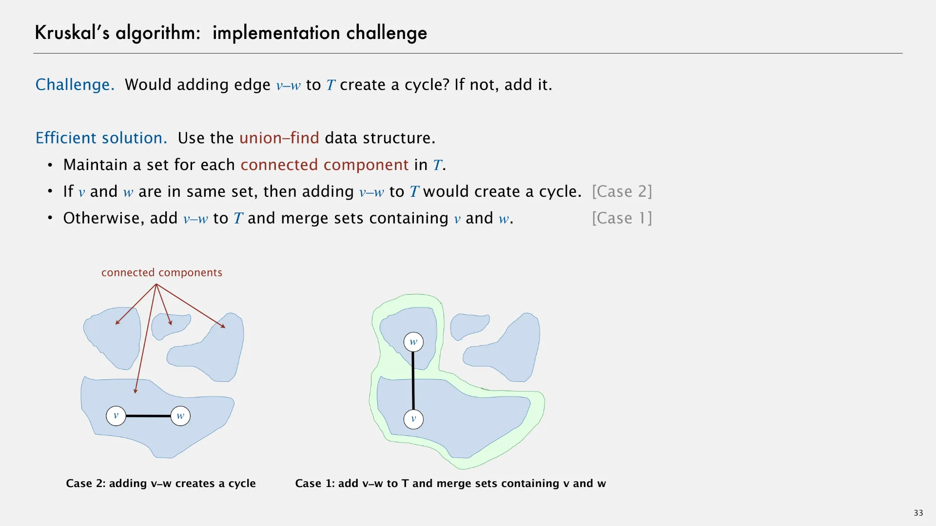
In case 2 (on the left of the above slide), adding an edge v-w creates a cycle within a connected component. In case 1 (on the right of the above slide), adding an edge v-w merges two connected components, forming a larger connected component.
Disjoint sets abstract data type
The disjoint sets (aka union-find) abstract data type is used to maintain the state of connected components. Specifically, our disjoint sets data type stores all the vertices in a graph as elements. A Java interface for disjoint sets might include two methods.
find(v)- Returns the representative for the given vertex. In Kruskal’s algorithm, we only add the current edge to the result if
find(v) != find(w). union(v, w)- Connects the two vertices v and w. In Kruskal’s algorithm, we use this to keep track of the fact that we joined the two connected components.
Using this DisjointSets data type, we can now implement Kruskal’s algorithm.
kruskalMST(Graph<V> graph) {
    // Create a DisjointSets implementation storing all vertices
    DisjointSets<V> components = new DisjointSetsImpl<V>(graph.vertices());
    // Get the list of edges in the graph
    List<Edge<V>> edges = graph.edges();
    // Sort the list of edges by weight
    edges.sort(Double.comparingDouble(Edge::weight));

    List<Edge<V>> result = new ArrayList<>();
    int i = 0;
    while (result.size() < graph.vertices().size() - 1) {
        Edge<V> e = edges.get(i);
        if (!components.find(e.from).equals(components.find(e.to))) {
            components.union(e.from, e.to);
            result.add(e);
        }
        i += 1;
    }
    return result;
}
The remainder of this lesson will focus on how we can go about implementing disjoint sets.
Look-over the following slides where Robert Sedgewick and Kevin Wayne introduce 3 ways of implementing the disjoint sets (union-find) abstract data type.
- Quick-find
- Optimizes for the
findoperation. - Quick-union
- Optimizes for the
unionoperation, but doesn’t really succeed.
- Weighted quick-union
- Addresses the worst-case height problem introduced in quick-union.
Quicksort
- Compare comparison sorting algorithms on efficiency and stability.
- Given the runtime of a partitioning algorithm, describe the runtime of quicksort.
- Describe the search trees analogies for quicksort algorithms.
Isomorphism not only inspires new ideas for data structures, but also new ideas for algorithms too. In our study of sorting algorithms, we learned that a sorting algorithm is considered stable if it preserves the original order of equivalent keys. Which sorting algorithms does Java use when you call Arrays.sort? It depends on whether we need stability.
- Stable system sort
- When sorting an array of objects (like emails), Java uses a sorting algorithm called Timsort, which is based on merge sort and has the same linearithmic worst-case runtime as merge sort.
Why is Timsort preferred over merge sort if they have the same worst-case runtime?
Timsort has the same worst-case asymptotic runtime as merge sort, but in experimental analysis it is often noticeably faster. It also has a linear-time best-case asymptotic runtime.
Timsort is a hybrid sort that combines ideas from merge sort with insertion sort. Experimental analysis reveals that the fastest sorting algorithm for small arrays is often insertion sort. Instead of merge sort’s base case of 1 element, Java Timsort uses a base case of 32 elements which are then insertion sorted. Insertion sort can be further sped up by using binary search to find the insertion point for the next unsorted element.
Timsort is also an adaptive sort that changes behavior depending on the input array. Many real-world arrays are not truly random. They often contain natural runs, or sorted subsequences of elements that could be efficiently merged. Rather than recursively dividing top-down, Timsort works bottom-up by identifying natural runs in the input array and combining them from left to right.
- Unstable system sort
- When sorting an array of numbers or booleans, Java uses a sorting algorithm called quicksort. Quicksort has many variants, but we’ll focus on two in this course:
- Single-pivot quicksort, which is isomorphic to binary search trees.
- Dual-pivot quicksort, which is like a 2-3 tree that only contains 3-nodes.
Partitioning
Quicksort relies on the idea of recursively partitioning an array around a pivot element, data[i].
A partitioning of an array rearranges its elements in a weaker way than sorting by requiring elements in the order:
- All elements to the left of the pivot are less than or equal to the pivot element.
- The pivot element,
data[i], moves to positionj. (The pivot might not need to move.) - All elements to the right of the pivot are greater than or equal to the pivot element.
Single-pivot quicksort
Partitioning an array around a pivot element in quicksort is like selecting a root element in a binary search tree. All the elements in the left subtree will be less than the root element, and all the elements in the right subtree will be greater than the root element.

The quicksort on the left always chooses the leftmost element as the pivot element and uses an ideal partitioning that maintains the relative order of the remaining elements. The binary search tree on the right shows the result of inserting each element in the left-to-right input order given by the array.
Open the VisuAlgo module to visualize sorting algorithms. Press
Escto exit the e-Lecture Mode, and choose QUI from the top navigation bar to switch to quicksort. Run the sorting algorithm using Sort from the bottom left menu.Note that the visualization does not use an ideal partitioning algorithm for quicksort.
Dual-pivot quicksort
Dual-pivot quicksort chooses 2 pivots on each recursive call, just like how 3-child nodes in 2-3 trees maintain 2 keys and 3 children. If choosing 1 pivot element is like choosing 1 root element in a binary node, then choosing 2 pivot elements is like choosing 2 root elements in a 3-child node.
Strictly speaking, dual-pivot quicksort is not isomorphic to 2-3 trees because there does not exist a one-to-one correspondence. Consider 2-3 trees that only contain 2-child nodes: the corresponding quicksort is single-pivot quicksort, not dual-pivot quicksort.
Partitioning an array around 2 pivot elements, p1 and p2 where p1 ≤ p2, rearranges its elements by requiring elements in the order:
- All elements less than p1.
- The pivot element p1.
- All elements x where p1 ≤ x ≤ p2.
- The pivot element p2.
- All elements greater than p2.
Dual-pivot quicksort is a relatively new algorithm published in 2009. Experimental analysis revealed that dual-pivot quicksort is significantly faster than single-pivot quicksort on modern computers. Computer scientists attribute the performance improvement due to advances in CPU caching and memory hierarchy since the 1960s and 1970s when single-pivot quicksort was first introduced.
Robert Sedgewick and Kevin Wayne. 2022. Minimum Spanning Trees. In COS 226: Spring 2022. ↩