Hashing and Graphs

Hash tables, affordance analysis, and graph data type.

Hash Tables
Affordance Analysis
Graph Data Type

Hash Tables

Explain and trace hash table algorithms such as insertion and search.
Evaluate how a hash table will behave in response to a given data type.
Analyze the runtime of a hash table with a given bucket data structure.

Java’s TreeSet and TreeMap classes are implemented using red-black trees that guarantee logarithmic time for most individual element operations. This is a massive improvement over sequential search: a balanced search tree containing over 1 million elements has a height on the order of about 20!

But it turns out that we can do even better by studying Java’s HashSet and HashMap classes, which are implemented using hash tables. Under certain conditions, hash tables can have constant time for most individual element operations—regardless of whether your hash table contains 1 million, 1 billion, 1 trillion, or even more elements.

Data-indexed integer set case study

Arrays store data contiguously in memory where each array index is next to each other. Unlike linked lists, arrays do not need to follow references throughout memory. Indexing into an array is a constant time operation as a result.

DataIndexedIntegerSet uses this idea of an array to implement a set of integers. It maintains a boolean[] present of length 2 billion, one index for almost every non-negative integer. The boolean value stored at each index present[x] represents whether or not the integer x is in the set.

void add(int x): Adds x to the set by assigning present[x] = true.
boolean contains(int x): Returns the value of present[x].
void remove(int x): Removes x from the set by assigning present[x] = false.

While this implementation is simple and fast, it takes a lot of memory to store the 2-billion length present array—and it doesn’t even work with negative integers or other data types. How might we generalize this concept to support strings?

Data-indexed string set case study

Let’s design a DataIndexedStringSet using a 27-element array: 1 array index for each lowercase letter in the English alphabet starting at index 1. A word starting with the letter ‘a’ goes to index 1, ‘b’ goes to index 2, ‘c’ goes to index 3, etc. To study the behavior of this program, let’s consider these three test cases.

DataIndexedStringSet set = new DataIndexedStringSet();
set.add("cat");

System.out.println(set.contains("car"));

DataIndexedStringSet set = new DataIndexedStringSet();
set.add("cat");

set.add("car");
set.remove("cat");
System.out.println(set.contains("car"));

DataIndexedStringSet set = new DataIndexedStringSet();
set.add("cat");

set.add("dog");
System.out.println(set.contains("dog"));

Some of the test cases work as we would expect a set to work, but other test cases don’t work.

Which of these test cases will behave correctly?

Only the third test case works as expected. “cat” and “car” collide because they share the same index, so changes to “cat” will also affect “car” and vice versa. This is unexpected because the set should treat the two strings as different from each other, but it turns out that changing the state of one will also change the state of the other.

A collision occurs when two or more elements share the same index. One way we can avoid collisions in a DataIndexedStringSet is to be more careful about how we assign each English word. If we make sure every English word has its own unique index, then we can avoid collisions!

Suppose the string “a” goes to 1, “b” goes to 2, “c” goes to 3, …, and “z” goes to 26. Then the string “aa” should go to 27, “ab” to 28, “ac” to 29, and so forth. Since there are 26 letters in the English alphabet, we call this enumeration scheme base 26. Each string gets its own number, so as strings get longer and longer, the number assigned to each string grows larger and larger as well.

Using base 26 numbering, we can compute the index for “cat” as (3 ∙ 26²) + (1 ∙ 26¹) + (20 ∙ 26⁰) = 2074. Breaking down this equation, we see that “cat” is a 3-letter word so there are 3 values added together:

(3 ∙ 26²): 3 represents the letter ‘c’, which is the 3rd letter in the alphabet.; 26 is raised to the 2nd power for the two subsequent letters.
(1 ∙ 26¹): 1 represents the letter ‘a’, which is the 1st letter in the alphabet.; 26 is raised to the 1st power for the one subsequent letter.
(20 ∙ 26⁰): 20 represents the letter ‘t’, which is the 20th letter in the alphabet.; 26 is raised to the 0th power for the zero subsequent letters.

So long as we pick a base that’s at least 26, this hash function is guaranteed to assign each lowercase English word a unique integer. But it doesn’t work with uppercase characters or punctuation. Furthermore, if we want to support other languages than English, we’ll need an even larger base. For example, there are 40,959 characters in the Chinese language alone. If we wanted to support all the possible characters in the Java built-in char type—which includes emojis, punctuation, and characters across many languages—we would need base 65536. Hash values generated this way will grow exponentially with respect to the length of the string!

Separate chaining hash tables

In practice, collisions are unavoidable. Instead of trying to avoid collisions by assigning a unique number to each element, separate chaining hash tables handle collisions by replacing the boolean[] present with an array of buckets, where each bucket can store zero or more elements.

Since separate chaining addresses collisions, we can now use smaller arrays. Instead of directly using the hash code as the index into the array, take the modulus of the hash code to compute an index into the array. Separate chaining turns the process from a single step to multiple steps:

Call the hash function on the given element to get a hash code, aka the number for that element.
Compute the bucket index by taking the modulus of the hash code by the array length.
Search the bucket for the given element.

Separate chaining comes with a cost. The worst case runtime for adding, removing, or finding an item is now in Θ(Q) where Q is the size of the largest bucket.

In general, the runtime of a separate chaining hash table is determined by a number of factors. We’ll often need to ask a couple of questions about the hash function and the hash table before we can properly analyze or predict the data structure performance.

What is the hash function’s likelihood of collisions?
What is the strategy for resizing the hash table.
What is the runtime for searching the bucket data structure.

To make good on our promise of a worst case constant time data structure for sets and maps, here’s the assumptions we need to make.

Assume the hash function distributes items uniformly.
Assume the hash table resizes by doubling, tripling, etc. upon exceeding a constant load factor.
Assume we ignore the time it takes to occasionally resize the hash table.

Affordance Analysis

Describe how abstractions can embody values and structure social relations.
Identify the affordances of a program abstraction such as a class or interface.
Evaluate affordances by applying the 3 value-sensitive design principles.

In the previous module focusing on implementing tree data structures and studying sorting algorithms, we learned methods for runtime analysis in order to help us evaluate the quality of an idea. The goal of runtime analysis was to produce a (1) predictive and (2) easy-to-compare description of the running time of an algorithm.

For the remaining half of the course, we’ll be studying a different category of data structures and algorithms called graphs. Unlike the study of tree data structures and sorting algorithms that focused on abstract inputs, the study of graph data structures and graph algorithms is often closely coupled with discussions about real-world data and problems. Runtime analysis will remain an important tool, but we also need methods of analysis to address questions at the intersection of algorithm design and the social responsibility that comes with it.

Affordance analysis is a method of analysis that measures which actions and outcomes that an abstraction makes more likely (affordances), and then evaluates the effects of these affordances on people and power hierarchies.

Affordances: Properties of objects that make specific outcomes more likely through the possible actions that it presents to users. In the context of designed physical objects, for example, a screwdriver affords turning screws (what it was designed for) but also affords other uses like digging narrow holes for planting seeds.; Likewise, disaffordances are properties that make certain outcomes less likely through the possible actions that it presents to users. A screwdriver disaffords ladling soup.

Affordance analysis is a process composed of two steps. First, identify affordances for the specific outcomes that they make more likely. Then, evaluate affordances according to how they shape social relations in particular applications.

Identify affordances

In Java, a class or interface defines public methods that afford certain actions. Many of these actions will seem quite value-neutral when defined in isolation from potential applications. For example:

We can add, remove, or check for an item at a given index in a list.
We can add, removeMin, or peekMin from a priority queue according to their priority values.
In Autocomplete, the allMatches method returns a list of all terms that match the given prefix.

In “The Limits of Correctness” (1985), Brian Cantwell Smith observes that a “correct” program is really only correct with respect to the programmer’s model of the problem:

When you design and build a computer system, you first formulate a model of the problem you want it to solve, and then construct the computer program in its terms. For example, if you were to design a medical system to administer drug therapy, you would need to model a variety of things: the patient, the drug, the absorption rate, the desired balance between therapy and toxicity, and so on and so forth. The absorption rate might be modelled as a number proportional to the patient’s weight, or proportional to body surface area, or as some more complex function of weight, age, and sex.

The choice of which model to use—such as (1) patient weight, (2) body surface area, or (3) weight + age + sex—encodes ideas about what is relevant or irrelevant. The results of software programs are determined by what and how we choose to model the problem.

Programming is the manipulation of this model by using calculation to change the rules and representations “at some particular level of abstraction […] So the drug model mentioned above would probably pay attention to the patients’ weight, but ignore their tastes in music.” When we choose to use certain data structures or algorithms, we are choosing to the model the problem in a certain way at a particular level of abstraction. We decide what is relevant or irrelevant in the model.

For example, we might ask: What are some affordances of comparison sorting algorithms? In comparison sorting, elements are rearranged according to an ordering relation defined by the compareTo method. It is assumed that these pairwise comparisons can be used to order all the elements on a line from least to greatest.

A Science and Technology Studies (STS) perspective might even suggest that sorting in and of itself—before any specific examples are introduced—is value-laden because sorting implies a way to order items on a line. Implementing compareTo is like assigning student grades: it takes all the complex dimensions of a human being and reduces them to a number compared against other peoples’ numbers. Using a sorting algorithm requires a programmer to select the aspects of an object that are most desirable for the task. This can be especially morally problematic when it is done without consent.

Value-sensitive design

Data is a key part of affordance analysis. But you might have noticed that your computing education rarely actually considers data on its own merit:

When verifying the correctness of your programs, we write code that generates dummy data or reads an example dataset without explanation about the data, who or what it aims to represent, and why the data was chosen.
When analyzing the running time of your programs, data matters to the extent that it helps us in case analysis, asymptotic analysis, or experimental analysis. Data is reduced to variables like N or abstract inputs.

To evaluate affordances, we will need to think about how each affordance interacts with the world by thinking through more realistic data and problems.

It helps to understand how managers, designers, and engineers are already thinking about the social implications of technologies. One framework for thinking through design is value-sensitive design (VSD), a “theory and method that accounts for human values in a principled and structured manner throughout the design process.”

Technologies that benefit some people can harm others. Batya Friedman, a Professor in the iSchool and one of the inventors of the method, surfaces this in a value scenario for SafetyNet, an imaginary service that helps people avoid “unsafe” areas.

SafetyNet is not just a hypothetical either. David Ingram and Cyrus Farivar write for NBC News: “Inside Citizen: The public safety app pushing surveillance boundaries.” It wouldn’t be hard to imagine a future where UW Alert partners with a tech company to create an app with functions similar to SafetyNet.

This SafetyNet value scenario imagines what the future could hold for different peoples and how the introduction of a technology changes how people behave. Batya’s value scenario highlights several different perspectives in evaluating a system by:

foregrounding human values (what is important to people in their lives),
considering the impacts of pervasive uptake (adoption, usage) of a technology,
and identifying direct and indirect stakeholders (people with concern or interest).

What kinds of human values could we consider? Batya suggests, as a starting point: privacy, trust, security, safety, community, freedom from bias, autonomy, identity, ownership, freedom of expression, dignity, calmness, compassion, respect, peace, wildness, sustainability, healing.

One key idea in this framework is the concept of value tensions: that human values do not exist in isolation and instead involve a balance between values that can come into tension when considering different individuals, groups, or societies. The goal of thinking through value tensions is to recognize the diverse values that exist in tension and work toward solutions that can engage with all of them.

Evaluate affordances

Whereas Batya’s SafetyNet value scenario focuses more on the large-scale overall product design, in this class, we focus on the details of how programs are implemented. As designers and implementers of interfaces, we might wonder about our responsibility in thinking through social implications.

Earlier, we identified that in the Autocomplete interface, the allMatches method returns a list of all terms that match the given prefix. Note that the method does not guarantee any particular order of results.

List<CharSequence> allMatches(CharSequence prefix)

How might we evaluate autocomplete in Husky Maps using the value-sensitive design perspectives?

Human values: The list of results produced by autocomplete provides users with everything that matches their search query. But the Autocomplete interface does not personalize these results at all: given a search query, everyone sees the same results. There is no parameter or field for storing the personalization information. Results could be more helpful if they were tuned to your profile.; Personalization, however, is not always a win. Personalization requires personal data that, in some cases, people may not actually want to disclose even if they “Agree” to the terms and conditions of using an app. Also, the value of convenience and helpfulness to the individual user can conflict with the goal of everyone receiving the same information. Hyper-personalized content feeds can lead to two people receiving drastically different information about the world.
Pervasive uptake: When everyone sees the same results, there can be material impacts if money and attention is directed in ways that reinforce existing social inequities. If everyone follows the same first-few suggestions, then we drive money and attention to those few places. This can also have downstream effects on public policy if it changes our perceptions of what we think of as important or valuable places. For example, public spaces like parks might lose our attention (and, therefore, public funding) if our app never recommended them.
Direct and indirect stakeholders: We can certainly imagine different situations around who might receive benefits or harms from the pervasive uptake of this technology. You can draw different examples by thinking about how different datasets could lead to different outcomes. Another perspective is to think about who does the work of managing or inputting the data. Is the data on places provided by the government, by individual owners of each place, by volunteers gathering data from the world? How might people want to change how places are represented or named in the app? Who is given the right to make these decisions?

You could also apply this same set of perspectives but instead focus on sorting the output list. Sorting requires selecting an abstraction for objects so that they can be ordered on a line. Husky Maps sorts autocomplete suggestions using importance values from the OpenStreetMap project. Combining these two pieces of information (the affordances of sorting and the example dataset) can lead to another affordance analysis.

Thinking through each perspective separately can help you assemble a more cohesive argument that considers the different potential impacts of software design. But in your final affordance analysis, you might find that your arguments combine ideas from 2 or all 3 perspectives. This recognizes the interconnectedness between the different ideas in your analysis.

Beyond value-sensitive design

Value-sensitive design, however, is just one theory or method for evaluating a technology. In Design Justice, Sasha Costanza-Chock critiques VSD:

VSD is descriptive rather than normative: it urges designers to be intentional about encoding values in designed systems but does not propose any particular set of values at all, let alone an intersectional understanding of racial, gender, disability, economic, environmental, and decolonial justice. VSD never questions the standpoint of the professional designer, doesn’t call for community inclusion in the design process (let alone community accountability or control), and doesn’t require an impact analysis of the distribution of material and symbolic benefits that are generated through design. Values are treated as disembodied abstractions, to be codified in libraries from which designers might draw to inform project requirements. In other words, in VSD we are meant to imagine that incorporating values into design can be accomplished largely by well-meaning expert designers.

VSD helped us think about data and problems on their own merit rather than as abstract concepts. But, in presenting evaluation as a process for designers to just think-through and analyze on their own—without consulting real people—values are treated as abstract concepts rather than situated in real human experiences.

If you’d like to learn more approaches to evaluating affordances, consider taking courses in (1) human–computer interaction, (2) qualitative research methods, or (3) community-engaged research.

Graph Data Type

Graph.java Digraph.java

Identify the features and representation for an example graph or graph problem.
Analyze the runtime of a graph representation in terms of vertices and edges.
Analyze the affordances of a graph interface or method for a particular problem.

Most of the data structures we’ve seen so far organize elements according to the properties of data in order to implement abstract data types like sets, maps, and priority queues.

Search trees use the properties of an element to determine where it belongs in the search tree. In TreeSet and TreeMap, the ordering relation is defined by the key’s compareTo.
Binary heaps compare the given priority values to determine whether to sink or swim a node in the heap. In PriorityQueue, the priority values are also defined by the key’s compareTo.
Hash tables use the properties of an element to compute a hash value, which then determines the bucket index. In HashSet and HashMap, the hash function is defined by the key’s hashCode.

All these data structures rely on properties of data to achieve efficiency. Checking if an element is stored in a balanced search tree containing 1 billion elements only requires about 30 comparisons—which sure beats having to check all 1 billion elements in an unsorted array. This is only possible because (1) the compareTo method defines an ordering relation and (2) the balanced search tree maintains log N height for any assortment of N elements.

But if we step back, all of this happens within the internal implementation details of the balanced search tree. Clients or other users of a balanced search tree treat it as an abstraction, or a structure that they can use without knowing its implementation details. In fact, the client can’t assume any particular implementation because they’re writing their code against more general interfaces like Set, Map, or Autocomplete.

Graphs, however, represent a totally different kind of abstract data type with different goals. Rather than focus on enabling efficient access to data, graphs focus on representing client-defined relationships between data.

Although graphs may look like weirdly-shaped trees, they are used in very different situations. The greatest difference lies in how a graph is used by a client. Instead of only specifying the element to add in a graph, we often will also specify the edges or relationships between elements too. Much of the usefulness of a graph comes from the explicit relationships between elements.

Husky Maps

In the Husky Maps case study, the MapGraph class represents all the streets in the Husky Maps app. Let’s focus on how data is represented in a graph.

public class MapGraph {
    private final Map<Point, List<Edge<Point>>> neighbors;
}

Here’s a breakdown of the data type for the neighbors variable:

Map<Point, List<Edge<Point>>>: A map where the keys are unique Point objects, and the values are the “neighbors” of each Point.
Point: An object that has an x coordinate and a y coordinate. Each point can represent a physical place in the real world, like a street intersection.
List<Edge<Point>>: A list of edges to other points. Each key is associated with one list of values; in other words, each Point is associated with a list of neighboring points.

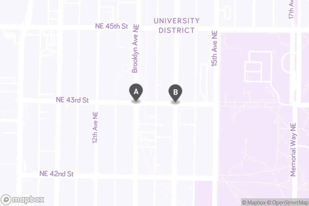
U District map with two markers on NE 43rd St

In this image, the Point labeled A represents the intersection Brooklyn Ave NE & NE 43rd St while the Point labeled B represents the intersection University Way NE & NE 43rd St. We say that the two points are “neighbors” because there’s a stretch of NE 43rd St in front of the light rail station that directly connects the two points.

More generally, a graph is a data type composed of vertices and edges defined by the client. In Husky Maps, the vertices are unique Point objects while the edges are stretches of road connecting points. Street intersections are connected to other street intersections. Unlike lists, deques, sets, maps, and priority queues that are defined largely by how they organize elements, graphs are defined by vertices and edges that define relationships between vertices.

In MapGraph, we included an edge representing the stretch of NE 43rd St in front of the light rail station. But this stretch of road is only accessible to buses, cyclists, and pedestrians. Personal vehicles are not allowed on this stretch of road, so the inclusion of this edge suggests that this graph would afford applications that emphasize public transit, bicycling, or walking. Graph designers make key decisions about what data is included and represented in their graph, and these decisions affect what kinds of problems can be solved.

Vertices and edges

Vertex (node): A basic element of a graph.; In MapGraph, vertices are represented using the Point class.
Edge: A direct connection between two vertices v and w in a graph, usually written as (v, w). Optionally, each edge can have an associated weight.; In MapGraph, edges are represented using the Edge class. The weight of an edge represents the physical distance between the two points adjacent to the edge.

Given a vertex, its edges lead to neighboring (or adjacent) vertices. In this course, we will always assume two restrictions on edges in a graph.

No self-loops. A vertex v cannot have an edge (v, v) back to itself.
No parallel (duplicate) edges. There can only exist at most one edge (v, w).

There are two types of edges.

Undirected edges: Represent pairwise connections between vertices allowing movement in both directions. Visualized as lines connecting two vertices.; In MapGraph, undirected edges are like two-way streets where traffic can go in both directions.
Directed edges: Represent pairwise connections between vertices allowing movement in a single direction. Visualized as arrows connecting one vertex to another.; In MapGraph, directed edges are like one-way streets.

Undirected graph abstract data type

An undirected graph (or simply “graph” without any qualifiers) is an abstract data type that contains zero or more vertices and zero or more undirected edges between pairs of vertices. The following slide¹ describes some undirected graph terminology.

Undirected graph terminology

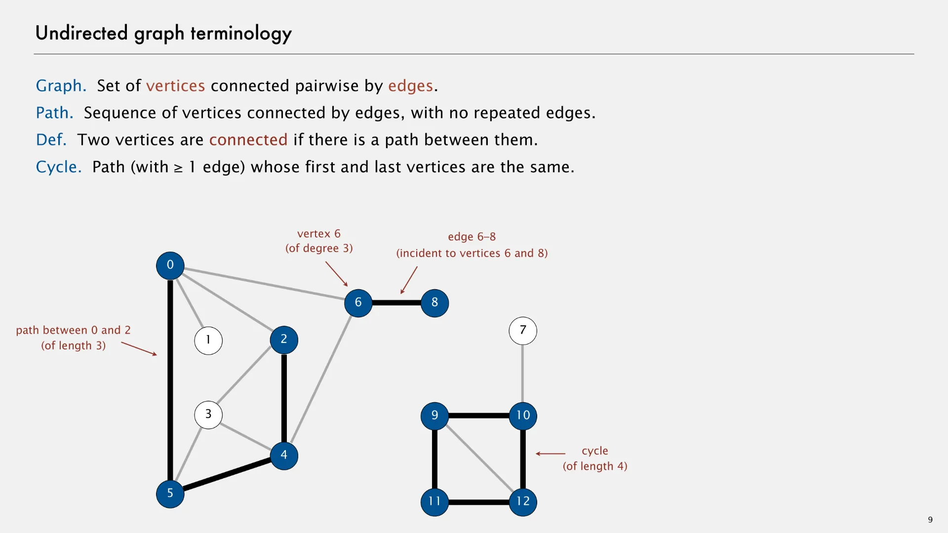
Path: Sequence of vertices connected by undirected edges, with no repeated edges.; Two vertices are connected if there is a path between them.
Cycle: Path (with 1 or more edges) whose first and last vertices are the same.
Degree: Number of undirected edges associated with a given vertex.

An interface for an undirected graph could require an addEdge and neighbors method.

public interface UndirectedGraph<V> {

    /** Add an undirected edge between vertices (v, w). */
    public void addEdge(V v, V w);

    /** Returns a list of the edges adjacent to the given vertex. */
    public List<Edge<V>> neighbors(V v);
}

Directed graph abstract data type

A directed graph (or “digraph”) is an abstract data type that contains zero or more vertices and zero or more directed edges between pairs of vertices. The following slide¹ describes some directed graph terminology.

Directed graph terminology

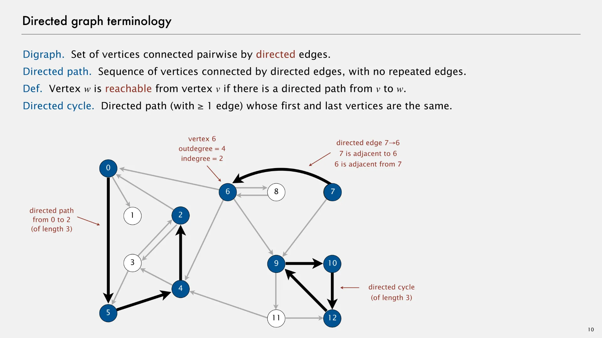
Although parallel (duplicate) edges are not allowed, a directed graph can have edges in both directions between each pair of nodes. In the example above, note there are edges (2, 3) and (3, 2), as well as edges (6, 8) and (8, 6). These two pairs of edges allow for movement in both directions.

Directed path: Sequence of vertices connected by directed edges, with no repeated edges.; Vertex w is reachable from vertex v if there is a directed path from v to w.
Directed cycle: Directed path (with 1 or more edges) whose first and last vertices are the same.
Outdegree: Number of directed edges outgoing from a given vertex.
Indegree: Number of directed edges incoming to the given vertex.

An interface for an directed graph could also require an addEdge and neighbors method, just as in the undirected graph example.

public interface DirectedGraph<V> {

    /** Add an directed edge between vertices (v, w). */
    public void addEdge(V v, V w);

    /** Returns a list of the outgoing edges from the given vertex. */
    public List<Edge<V>> neighbors(V v);
}

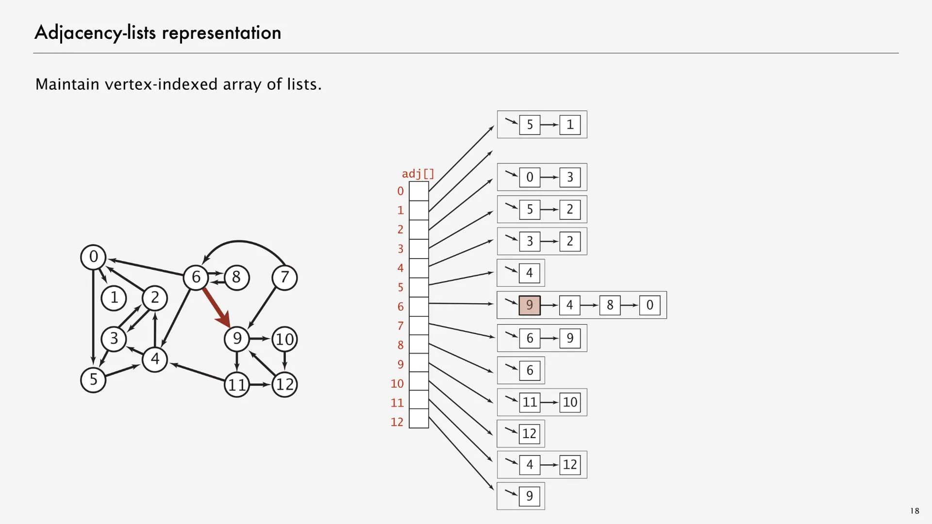
Adjacency lists data structure

Adjacency lists is a data structure for implementing both undirected graphs and directed graphs.

Adjacency lists: A graph data structure that associates each vertex with a list of edges.

MapGraph uses an adjacency lists data structure: the neighbors map associates each Point with a List<Edge<Point>>. The adjacency lists provides a very direct implementation of the DirectedGraph interface methods like addEdge and neighbors.

public class MapGraph implements DirectedGraph<Point> {
    private final Map<Point, List<Edge<Point>>> neighbors;

    /** Constructs a new map graph. */
    public MapGraph(...) {
        neighbors = new HashMap<>();
    }

    /** Adds a directed edge to this graph using distance as weight. */
    public void addEdge(Point from, Point to) {
        if (!neighbors.containsKey(from)) {
            neighbors.put(from, new ArrayList<>());
        }
        neighbors.get(from).add(new Edge<>(from, to, estimatedDistance(from, to)));
    }

    /** Returns a list of the outgoing edges from the given vertex. */
    public List<Edge<Point>> neighbors(Point point) {
        if (!neighbors.containsKey(point)) {
            return new ArrayList<>();
        }
        return neighbors.get(point);
    }
}

The MapGraph class doesn’t have a method for adding just a single vertex or getting a list of all the vertices or all the edges. These aren’t necessary for Husky Maps. But in other situations, you might like having these methods that provide different functionality. The Java developers did not provide a standard Graph interface like they did for List, Set, or Map because graphs are often custom-designed for specific problems. What works for Husky Maps might not work well for other graph problems.

There are many options for Map and Set implementations. Instead of HashMap, we could have chosen TreeMap; instead of HashSet, TreeSet. However, we’ll often visualize adjacency lists by drawing the map as an array associating each vertex with a linked list representing its neighbors. The following graph visualization¹ on the left matches with the data structure visualization on the right, with the edge (6, 9) marked red in both the left and the right side.

Adjacency lists representation

Adjacency lists aren’t the only way to implement graphs. Two other common approaches are adjacency matrices and edge sets. Both of these approaches provide different affordances (making some graph methods easier to implement or more efficient in runtime), but adjacency lists are still the most popular option for the graph algorithms we’ll see in this class. Keith Schwarz writes on StackOverflow about a few graph problems where you might prefer using an adjacency matrix over an adjacency list but summarizes at the top:

Adjacency lists are generally faster than adjacency matrices in algorithms in which the key operation performed per node is “iterate over all the nodes adjacent to this node.” That can be done in time O(deg(v)) time for an adjacency list, where deg(v) is the degree of node v, while it takes time Θ(n) in an adjacency matrix. Similarly, adjacency lists make it fast to iterate over all of the edges in a graph—it takes time O(m + n) to do so, compared with time Θ(n²) for adjacency matrices.
Some of the most-commonly-used graph algorithms (BFS, DFS, Dijkstra’s algorithm, A* search, Kruskal’s algorithm, Prim’s algorithm, Bellman-Ford, Karger’s algorithm, etc.) require fast iteration over all edges or the edges incident to particular nodes, so they work best with adjacency lists.

Robert Sedgewick and Kevin Wayne. 2020. Graphs and Digraphs. ↩ ↩² ↩³