Graph Algorithms
Graph traversals, SPTs, and Dynamic Programming.
Graph Traversals
BreadthFirstPaths.javaDepthFirstPaths.java
- Trace and explain each data structure in BFS and DFS graph traversal.
- Analyze the runtime of a graph algorithm in terms of vertices and edges.
- Define an appropriate graph abstraction for a given image processing problem.
How do we use a graph to solve problems like computing navigation directions? Before we can discuss graph algorithms, we’ll need a way to traverse a graph or explore all of its data. To traverse a tree, we can start from the overall root and recursively work our way down. To traverse a hash table, we can start from bucket index 0 and iterate over all the separate chains. But for a graph, where do we start the traversal?
By applying the recursive tree traversal idea, we discovered a graph algorithm called depth-first search (DFS). Depth-first search isn’t the only graph traversal algorithm, and it’s often compared to another graph traversal algorithm called breadth-first search (BFS). BFS will be the template for many of the graph algorithms that we’ll learn in the coming lessons.
- Breadth-first search (BFS)
- An iterative graph traversal algorithm that expands outward, level-by-level, from a given
startvertex.void bfs(Graph<V> graph, V start) { Queue<V> perimeter = new ArrayDeque<>(); Set<V> visited = new HashSet<>(); perimeter.add(start); visited.add(start); while (!perimeter.isEmpty()) { V from = perimeter.remove(); // Process the current vertex by printing it out System.out.println(from); for (Edge<V> edge : graph.neighbors(from)) { V to = edge.to; if (!visited.contains(to)) { perimeter.add(to); visited.add(to); } } } } - Depth-first search (DFS)
- A recursive graph traversal algorithm that explores as far as possible from a given
startvertex until it reaches a base case and needs to backtrack.void dfs(Graph<V> graph, V start) { dfs(graph, start, new HashSet<>()); } dfs(Graph<V> graph, V from, Set<V> visited) { // Process the current vertex by printing it out System.out.println(from); visited.add(from); for (Edge<V> edge : graph.neighbors(from)) { V to = edge.to; if (!visited.contains(to)) { dfs(graph, to); } } }
BFS and DFS represent two ways of traversing over all the data in a graph by visiting all the vertices and checking all the edges. BFS and DFS are like the for loops of graphs: on their own, they don’t solve a specific problem, but they are an important building block for graph algorithms.
BFS provides a lot more utility than DFS in this context because it can be used to find the shortest paths in a unweighted graph with the help of two extra data structures called edgeTo and distTo.
Map<V, Edge<V>> edgeTomaps each vertex to the edge used to reach it in the BFS traversal.Map<V, Integer> distTomaps each vertex to the number of edges from thestartvertex.
We’ll study these two maps in greater detail over the following lessons.
Problems and solutions
Whereas sets, maps, and priority queues emphasize efficient access to elements, graphs emphasize not only elements (vertices) but also the relationships between elements (edges). The efficiency of a graph data structure depends on the underlying data structures used to represent its vertices and edges. But there’s another way to understand graphs through the lens of computational problems and algorithmic solutions.
- Computational problem
- An abstract problem that can be represented, formalized, and/or solved using algorithms.
- In Java, we often represent problems using interfaces describing expected functionality.
Sorting is the problem of rearranging elements according to an ordering relation (via comparison). Sets are an example of an abstract data type that represents a collection of unique elements. Graph traversal is the problem of visiting/checking/processing each vertex in a graph.
- Algorithmic solution
- A a sequence of steps or description of process that can be used to solve computational problems.
- In Java, we often represent solutions using classes detailing how to implement functionality.
Insertion sort, selection sort, and merge sort are algorithms for sorting. Search trees and hash tables are algorithms for implementing sets. BFS and DFS are algorithms for graph traversal.
This relationships suggests that problems like graph search can be represented using interfaces, which are then implemented by solutions that are represented using classes. In Husky Maps, the graphs.shortestpaths package includes interfaces and classes for finding the shortest paths in a directed graph.
public interface ShortestPathSolver<V>
public class DijkstraSolver<V> implements ShortestPathSolver<V>
public class BellmanFordSolver<V> implements ShortestPathSolver<V>
public class ToposortDAGSolver<V> implements ShortestPathSolver<V>
Each of these graph algorithms—Dijkstra’s algorithm, Bellman-Ford algorithm, and the toposort-DAG algorithm—do most of their work in the class constructor. If we wanted to add a BFS algorithm to this list, it would take the bfs method defined above and do most of the work inside of the constructor.
public class BreadthFirstSearch<V> {
    private final Map<V, Edge<V>> edgeTo;
    private final Map<V, Integer> distTo;

    public BreadthFirstSearch(Graph<V> graph, V start) {
        edgeTo = new HashMap<>();
        distTo = new HashMap<>();
        Queue<V> perimeter = new ArrayDeque<>();
        Set<V> visited = new HashSet<>();
        perimeter.add(start);
        visited.add(start);
        edgeTo.put(start, null);
        distTo.put(start, 0);
        while (!perimeter.isEmpty()) {
            V from = perimeter.remove();
            for (Edge<V> edge : graph.neighbors(from)) {
                V to = edge.to;
                if (!visited.contains(to)) {
                    edgeTo.put(to, edge);
                    distTo.put(to, distTo.get(from) + 1);
                    perimeter.add(to);
                    visited.add(to);
                }
            }
        }
    }

    /** Returns the unweighted shortest path from the start to the goal. */
    public List<V> solution(V goal) {
        List<V> path = new ArrayList<>();
        V curr = goal;
        path.add(curr);
        while (edgeTo.get(curr) != null) {
            curr = edgeTo.get(curr).from;
            path.add(curr);
        }
        Collections.reverse(path);
        return path;
    }
}
The solution method begins at goal and uses edgeTo to trace the path back to start.
There are hundreds of problems and algorithms for solving them. The field of graph theory investigates these graph problems and graph algorithms.
Topological sorting DAG algorithm
- Apply the DFS algorithm to create a topological sorted order of vertices.
Topological sorting is a graph problem for ordering all the vertices in a directed acyclic graph (DAG).
The algorithm that we’ll introduce to solve topological sorting doesn’t have a commonly-accepted name. The algorithm solves topological sorting by returning all the vertices in the graph in reverse DFS postorder:
- DFS
- Depth-first search.
- DFS postorder
- A particular way of running depth-first search. DFS is recursive, so we can process each value either before or after the recursive calls to all the neighbors. A preorder processes the value before the recursive calls while a postorder processes the value after the recursive calls.
- Reverse DFS postorder
- The DFS postorder list, but in backwards (reverse) order.
In the following visualization, notice how the first value in the DFS postorder is 4 because 4 has no outgoing neighbors! We then add 1 after visiting all of 1’s neighbors. And repeat!
In (forward) DFS postorder, we add the following vertices:
- The first vertex added to the
resultlist is like a leaf in a tree: it has no outgoing neighbors so it is not a “prerequisite” for any other vertex. - The second vertex added to the
resultlist points to the first vertex. - …
- The final vertex added to the
resultlist is the start vertex.
So the reverse DFS postorder has the first vertex (the “leaf”) at the end of the result list where it belongs in the topological sorting.
Topological sorting provides an alternative way to find a shortest paths tree in a directed acyclic graph (DAG) by relaxing edges in the order given by the topological sort. In class, we’ll learn more about the significance of this alternative approach and what it means in comparison to Dijkstra’s algorithm.
Shortest Paths Trees
- Trace Dijkstra’s algorithm for shortest paths trees.
- Explain why Dijkstra’s algorithm might not work with negative edge weights.
- Explain the runtime for Dijkstra’s algorithm in terms of priority queue operations.
Breadth-first search (BFS) can be used to solve the unweighted shortest paths problem, of which we’ve studied 3 variations:
- Single-pair shortest paths
- Given a source vertex s and target t, what is the shortest path from s to t?
- Single-source shortest paths
- Given a source vertex s what are the shortest paths from s to all vertices in the graph?
- Multiple-source shortest paths
- Given a set of source vertices S, what are the shortest paths from any vertex in S to all vertices in the graph.
In the context of BFS and unweighted shortest paths, the metric by which we define “shortest” is the number of edges on the path. But, in Husky Maps, we need a metric that is sensitive to the fact that road segments are not all the same length. In Husky Maps, the weight of an edge represents the physical distance of a road segment. Longer road segments have larger weight values than shorter road segments.
- Weighted shortest paths problem
- For the single pair variant: Given a source vertex s and target vertex t what is the shortest path from s to t minimizing the sum total weight of edges?
Dijkstra’s algorithm
Dijkstra’s algorithm is the most well-known algorithm for finding a weighted SPT in a graph.
Dijkstra’s algorithm gradually builds a shortest paths tree on each iteration of the while loop. The algorithm selects the next unvisited vertex based on the sum total cost of its shortest path.
public class DijkstraSolver<V> implements ShortestPathSolver<V> {
    private final Map<V, Edge<V>> edgeTo;
    // Maps each vertex to the weight of the best-known shortest path.
    private final Map<V, Double> distTo;

    /**
     * Constructs a new instance by executing Dijkstra's algorithm on the graph from the start.
     *
     * @param graph the input graph.
     * @param start the start vertex.
     */
    public DijkstraSolver(Graph<V> graph, V start) {
        edgeTo = new HashMap<>();
        distTo = new HashMap<>();

        MinPQ<V> perimeter = new DoubleMapMinPQ<>();
        perimeter.add(start, 0.0);

        // The shortest path from the start to the start requires no edges (0 cost).
        edgeTo.put(start, null);
        distTo.put(start, 0.0);

        Set<V> visited = new HashSet<>();

        while (!perimeter.isEmpty()) {
            V from = perimeter.removeMin();
            visited.add(from);

            for (Edge<V> edge : graph.neighbors(from)) {
                V to = edge.to;
                // oldDist is the weight of the best-known path not using this edge.
                double oldDist = distTo.getOrDefault(to, Double.POSITIVE_INFINITY);
                // newDist is the weight of the shortest path using this edge.
                double newDist = distTo.get(from) + edge.weight;
                // Check that we haven't added the vertex to the SPT already...
                // AND the path using this edge is better than the best-known path.
                if (!visited.contains(to) && newDist < oldDist) {
                    edgeTo.put(to, edge);
                    distTo.put(to, newDist);
                    perimeter.addOrChangePriority(to, newDist);
                }
                // This entire if block is called "relaxing" an edge.
            }
        }
    }

    /** Returns a single-pair weighted shortest path from start to goal. */
    public List<V> solution(V goal) {
        List<V> path = new ArrayList<>();
        V curr = goal;
        path.add(curr);
        while (edgeTo.get(curr) != null) {
            curr = edgeTo.get(curr).from;
            path.add(curr);
        }
        Collections.reverse(path);
        return path;
    }
}
This code works fine, but in practice, you’ll often see a similar version of this code that is basically the same except it makes no mention of the visited set. If we were to remove the visited set from BFS, BFS can get stuck in a loop or cause other kinds of problems. But Dijkstra’s algorithm actually runs the same with or without the visited set. In class, we’ll learn more about why this optimization works without causing any infinite loops.
Dynamic Programming
- Identify whether a recursive algorithm can be rewritten using DP.
- Explain how unique paths can be counted using recursion and DP.
- Explain how a min-cost seam can be found using recursion and DP.
Graph data structures (like adjacency lists) and graph algorithms (like Dijkstra’s algorithm) provided reusable abstractions for addressing many kinds of problems. Reduction refers to exactly this problem solving approach: modifying the input data to a problem so that an existing algorithm can solve it.
- Reduction
- A problem-solving approach that works by reframing problem A in terms of another problem B:
- Preprocess. Take the original input to A and modify it so that it works as an input to B.
- Run a standard algorithm for problem B on this input, returning some output.
- Postprocess. Modify this output so that it can be understood as the expected output for A.
We’ve actually already seen several examples of reduction algorithms that we just didn’t call “reductions” at the time. For example, in the project, we learned that seam finding reduces to single-pair shortest paths:
- First, we constructed a
PixelGraphfrom your inputPicture. - Then, we ran a shortest paths algorithm, returning the shortest path as a list of nodes.
- Finally, we extracted the y-index of each node representing the pixels in the seam to remove.
Reduction algorithms are a very common approach to solving problems in computer science. They also work without graphs as input or context. Remember dup1 and dup2 from the first week of the course? dup1 detects duplicates in an array by checking every pair of items in quadratic time. dup2 detects duplicates in a sorted array in just linear time. The problem of duplicate detection reduces to sorting because we can just sort the array and then run dup2, which can be much faster than dup1. Inventing faster sorting algorithms doesn’t just mean faster sorting, but faster everything because so many problems reduce to or otherwise depend on sorting.
Eric Allender summarizes the importance of this insight:1
If A is efficiently reducible to B, and B is efficiently reducible to A, then in a very meaningful sense, A and B are “equivalent”—they are merely two different ways of looking at the same problem. Thus instead of infinitely many different apparently unrelated computational problems, one can deal instead with a much smaller number of classes of equivalent problems […] Nothing had prepared the computing community for the shocking insight that there are really just a handful of fundamentally different computational problems that people want to solve.
Although reductions provide a powerful way to define classes of equivalent computational problems, they don’t necessarily lead to the most experimentally-efficient solutions. The seam finding reduction to single-pair shortest paths will be limited by the runtime for shortest paths algorithms like Dijkstra’s algorithm. In practice, algorithm designers apply algorithm design paradigms like dynamic programming to develop more efficient solutions when greater efficiency is necessary.
Fibonacci sequence case study
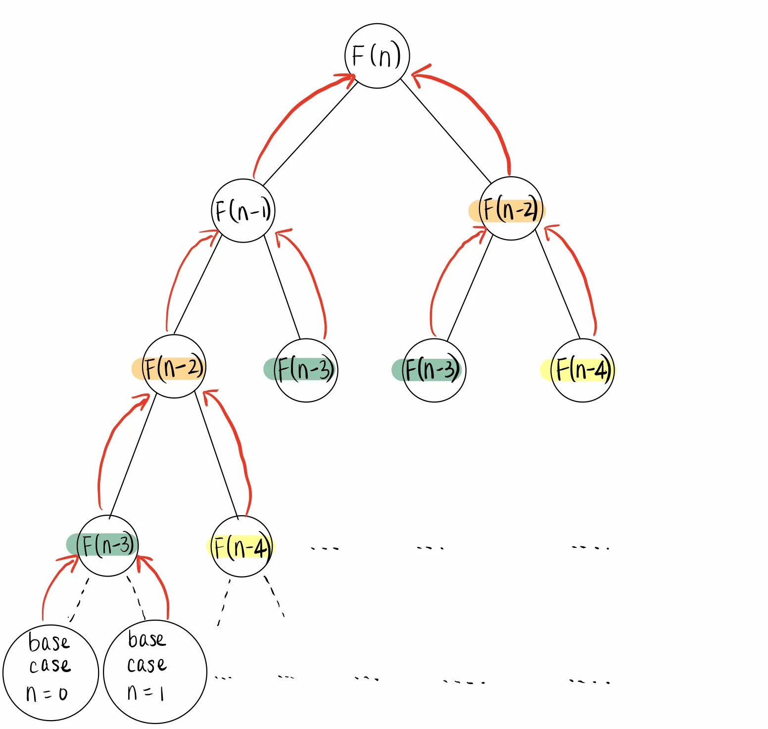
The Fibonacci Sequence is a series of numbers in which each number is the sum of the two preceding numbers, starting with 0 and 1. We can represent this rule as a recurrence: F(N) = F(N - 1) + F(N - 2) with the base cases F(0) = 0 and F(1) = 1.
By converting this recurrence into a program, we can compute the Nth Fibonacci number using multiple recursion.
public static long fib(int N) {
    if (N == 0 || N == 1) {
        return N;
    }
    return fib(N - 1) + fib(N - 2);
}
We can draw a recursion tree diagram to visualize the process for computing fib(N). Each node in the diagram represents a call to fib, starting from F(N), which calls F(N - 1) and F(N - 2). F(N - 1) then calls F(N - 2) and F(N - 3), and so forth. Repeated subproblems are highlighted in different colors.
Top-down dynamic programming
To save time, we can reuse the solutions to repeated subproblems. Top-down dynamic programming is a kind of dynamic programming that augments the multiple recursion algorithm with a data structure to store or cache the result of each subproblem. Recursion is only used to solve each unique subproblem exactly once, leading to a linear time algorithm for computing the Nth Fibonacci number.
private static long[] F = new long[92];

public static long fib(int N) {
    if (N == 0 || N == 1) {
        return N;
    }
    if (F[N] == 0) {
        F[N] = fib(N - 1) + fib(N - 2);
    }
    return F[N];
}
Top-down dynamic programming is also known as memoization because it provides a way to turn multiple recursion with repeated subproblems into dynamic programming by remembering past results.
| index | 0 | 1 | 2 | 3 | 4 | 5 | 6 |
|---|---|---|---|---|---|---|---|
| F(N) | 0 | 1 | 1 | 2 | 3 | 5 | 8 |
The data structure needs to map each input to its respective result. In the case of fib, the input is an int and the result is a long. Because the integers can be directly used as indices into an array, we chose to use a long[] as the data structure for caching results. But, in other programs, we may instead want to use some other kind of data structure like a Map to keep track of each input and result.
Bottom-up dynamic programming
Like top-down dynamic programming, bottom-up dynamic programming is another kind of dynamic programming that also uses the same data structure to store results. But bottom-up dynamic programming populates the data structure using iteration rather than recursion, requiring the algorithm designer to carefully order computations.
public static long fib(int N) {
    long[] F = new long[N + 1];
    F[0] = 0;
    F[1] = 1;
    for (int i = 2; i <= N; i += 1) {
        F[i] = F[i - 1] + F[i - 2];
    }
    return F[N];
}
After learning both top-down and bottom-up dynamic programming, we can see that there’s a common property between the two approaches.
- Dynamic programmming
- An algorithm design paradigm for speeding-up algorithms that makes multiple recursive calls by identifying and reusing solutions to repeated recursive subproblems.
Eric Allender. 2009. A Status Report on the P versus NP Question. ↩