Graph Algorithms

Shortest paths trees and dynamic programming.

1. Shortest Paths Trees
   1. Dijkstra’s algorithm
   2. Topological sorting DAG algorithm
2. Dynamic Programming
   1. Fibonacci sequence case study
   2. Top-down dynamic programming
   3. Bottom-up dynamic programming
3. Disjoint Sets
   1. Kruskal’s algorithm
   2. Disjoint sets abstract data type

Shortest Paths Trees

1. Trace Dijkstra’s and the topological sorting algorithm for shortest paths trees.
2. Explain why Dijkstra’s algorithm might not work with negative edge weights.
3. Explain the runtime for Dijkstra’s algorithm in terms of priority queue operations.

Breadth-first search (BFS) can be used to solve the unweighted shortest paths problem, of which we’ve studied 3 variations:

Single-pair shortest paths

Given a source vertex s and target t, what is the shortest path from s to t?

Single-source shortest paths

Given a source vertex s what are the shortest paths from s to all vertices in the graph?

Multiple-source shortest paths

Given a set of source vertices S, what are the shortest paths from any vertex in S to all vertices in the graph.

In the context of BFS and unweighted shortest paths, the metric by which we define “shortest” is the number of edges on the path. But, in Husky Maps, we need a metric that is sensitive to the fact that road segments are not all the same length. In Husky Maps, the weight of an edge represents the physical distance of a road segment. Longer road segments have larger weight values than shorter road segments.

Weighted shortest paths problem

For the single pair variant: Given a source vertex s and target vertex t what is the shortest path from s to t minimizing the sum total weight of edges?

In this lesson, we’ll learn about Dijkstra’s algorithm as a modification of Prim’s algorithm. It’s important to keep in mind that the algorithms are designed to find different kinds of trees. Watch this short visualization to see the difference.

Dijkstra’s algorithm

Dijkstra’s algorithm is the most well-known algorithm for finding a weighted SPT in a graph. Just as Prim’s algorithm built on the foundation of BFS, Dijkstra’s algorithm can be seen as a variation of Prim’s algorithm.

Dijkstra’s algorithm gradually builds a shortest paths tree on each iteration of the while loop. But whereas Prim’s algorithm selects the next unvisited vertex based on edge weight alone Dijkstra’s algorithm selects the next unvisited vertex based on the sum total cost of its shortest path. Review the comments in this code snippet to identify how this change appears in Dijkstra’s algorithm.

public class DijkstraSolver<V> implements ShortestPathSolver<V> {
    private final Map<V, Edge<V>> edgeTo;
    // Maps each vertex to the weight of the best-known shortest path.
    private final Map<V, Double> distTo;

    /**
     * Constructs a new instance by executing Dijkstra's algorithm on the graph from the start.
     *
     * @param graph the input graph.
     * @param start the start vertex.
     */
    public DijkstraSolver(Graph<V> graph, V start) {
        edgeTo = new HashMap<>();
        distTo = new HashMap<>();

        MinPQ<V> perimeter = new DoubleMapMinPQ<>();
        perimeter.add(start, 0.0);

        // The shortest path from the start to the start requires no edges (0 cost).
        edgeTo.put(start, null);
        distTo.put(start, 0.0);

        Set<V> visited = new HashSet<>();

        while (!perimeter.isEmpty()) {
            V from = perimeter.removeMin();
            visited.add(from);

            for (Edge<V> edge : graph.neighbors(from)) {
                V to = edge.to;
                // oldDist is the weight of the best-known path not using this edge.
                double oldDist = distTo.getOrDefault(to, Double.POSITIVE_INFINITY);
                // newDist is the weight of the shortest path using this edge.
                double newDist = distTo.get(from) + edge.weight;
                // Check that we haven't added the vertex to the SPT already...
                // AND the path using this edge is better than the best-known path.
                if (!visited.contains(to) && newDist < oldDist) {
                    edgeTo.put(to, edge);
                    distTo.put(to, newDist);
                    perimeter.addOrChangePriority(to, newDist);
                }
                // This entire if block is called "relaxing" an edge.
            }
        }
    }

    /** Returns a single-pair weighted shortest path from start to goal. */
    public List<V> solution(V goal) {
        List<V> path = new ArrayList<>();
        V curr = goal;
        path.add(curr);
        while (edgeTo.get(curr) != null) {
            curr = edgeTo.get(curr).from;
            path.add(curr);
        }
        Collections.reverse(path);
        return path;
    }
}

This code works fine, but in practice, you’ll often see a similar version of this code that is basically the same except it makes no mention of the visited set. If we were to remove the visited set from BFS or Prim’s algorithm, BFS and Prim’s algorithms can get stuck in a loop or cause other kinds of problems. But Dijkstra’s algorithm actually runs the same with or without the visited set. In class, we’ll learn more about why this optimization works without causing any infinite loops.

Topological sorting DAG algorithm

Topological sorting is a graph problem for ordering all the vertices in a directed acyclic graph (DAG).

The algorithm that we’ll introduce to solve topological sorting doesn’t have a commonly-accepted name. The algorithm solves topological sorting by returning all the vertices in the graph in reverse DFS postorder:

DFS

Depth-first search.

DFS postorder

A particular way of running depth-first search. DFS is recursive, so we can process each value either before or after the recursive calls to all the neighbors. A preorder processes the value before the recursive calls while a postorder processes the value after the recursive calls.

Reverse DFS postorder

The DFS postorder list, but in backwards (reverse) order.

public class ReverseDFSPostorderToposort<V> {
    private final List<V> result;

    public ReverseDFSPostorderToposort(Graph<V> graph) {
        result = new ArrayList<>();
        Set<V> visited = new HashSet<>();
        // Run the algorithm from all possible start points
        // if there are multiple disjoint parts of the graph.
        for (V start : graph.vertices()) {
            if (!visited.contains(start)) {
                dfsPostorder(graph, start, visited);
            }
        }
        // Reverse the DFS postorder.
        Collections.reverse(result);
    }

    private void dfsPostorder(Graph<V> graph, V from, Set<V> visited) {
        visited.add(from);
        for (Edge<V> edge : graph.neighbors(from)) {
            V to = edge.to;
            if (!visited.contains(to)) {
                dfsPostorder(graph, to, visited);
            }
        }
        // Postorder: Add current vertex after visiting all the neighbors
        result.add(from);
    }

    /** Returns a topological sorting of vertices in the graph. */
    public List<V> toposort() {
        return result;
    }
}

In the following visualization, notice how the first value in the DFS postorder is 4 because 4 has no outgoing neighbors! We then add 1 after visiting all of 1’s neighbors. And repeat!

In (forward) DFS postorder, we add the following vertices:

• The first vertex added to the result list is like a leaf in a tree: it has no outgoing neighbors so it is not a “prerequisite” for any other vertex.
• The second vertex added to the result list points to the first vertex.
• …
• The final vertex added to the result list is the start vertex.

So the reverse DFS postorder has the first vertex (the “leaf”) at the end of the result list where it belongs in the topological sorting.

Topological sorting provides an alternative way to find a shortest paths tree in a directed acyclic graph (DAG) by relaxing edges in the order given by the topological sort. In class, we’ll learn more about the significance of this alternative approach and what it means in comparison to Dijkstra’s algorithm.

Dynamic Programming

1. Identify whether a recursive algorithm can be rewritten using DP.
2. Explain how unique paths can be counted using recursion and DP.
3. Explain how a min-cost seam can be found using recursion and DP.

Graph data structures (like adjacency lists) and graph algorithms (like Dijkstra’s algorithm) provided reusable abstractions for addressing many kinds of problems. Reduction refers to exactly this problem solving approach: modifying the input data to a problem so that an existing algorithm can solve it.

Reduction

A problem-solving approach that works by reframing problem A in terms of another problem B:

1. Preprocess. Take the original input to A and modify it so that it works as an input to B.
2. Run a standard algorithm for problem B on this input, returning some output.
3. Postprocess. Modify this output so that it can be understood as the expected output for A.

We’ve actually already seen several examples of reduction algorithms that we just didn’t call “reductions” at the time. For example, in the project, we learned that seam finding reduces to single-pair shortest paths:

• First, we constructed a PixelGraph from your input Picture.
• Then, we ran a shortest paths algorithm, returning the shortest path as a list of nodes.
• Finally, we extracted the y-index of each node representing the pixels in the seam to remove.

Reduction algorithms are a very common approach to solving problems in computer science. They also work without graphs as input or context. Remember dup1 and dup2 from the first week of the course? dup1 detects duplicates in an array by checking every pair of items in quadratic time. dup2 detects duplicates in a sorted array in just linear time. The problem of duplicate detection reduces to sorting because we can just sort the array and then run dup2, which can be much faster than dup1. Inventing faster sorting algorithms doesn’t just mean faster sorting, but faster everything because so many problems reduce to or otherwise depend on sorting.

Eric Allender summarizes the importance of this insight:¹

If A is efficiently reducible to B, and B is efficiently reducible to A, then in a very meaningful sense, A and B are “equivalent”—they are merely two different ways of looking at the same problem. Thus instead of infinitely many different apparently unrelated computational problems, one can deal instead with a much smaller number of classes of equivalent problems […] Nothing had prepared the computing community for the shocking insight that there are really just a handful of fundamentally different computational problems that people want to solve.

Although reductions provide a powerful way to define classes of equivalent computational problems, they don’t necessarily lead to the most experimentally-efficient solutions. The seam finding reduction to single-pair shortest paths will be limited by the runtime for shortest paths algorithms like Dijkstra’s algorithm. In practice, algorithm designers apply algorithm design paradigms like dynamic programming to develop more efficient solutions when greater efficiency is necessary.

Fibonacci sequence case study

The Fibonacci Sequence is a series of numbers in which each number is the sum of the two preceding numbers, starting with 0 and 1. We can represent this rule as a recurrence: F(N) = F(N - 1) + F(N - 2) with the base cases F(0) = 0 and F(1) = 1.

By converting this recurrence into a program, we can compute the N^th Fibonacci number using multiple recursion.

public static long fib(int N) {
    if (N == 0 || N == 1) {
        return N;
    }
    return fib(N - 1) + fib(N - 2);
}

We can draw a recursion tree diagram to visualize the process for computing fib(N). Each node in the diagram represents a call to fib, starting from F(N), which calls F(N - 1) and F(N - 2). F(N - 1) then calls F(N - 2) and F(N - 3), and so forth. Repeated subproblems are highlighted in different colors.

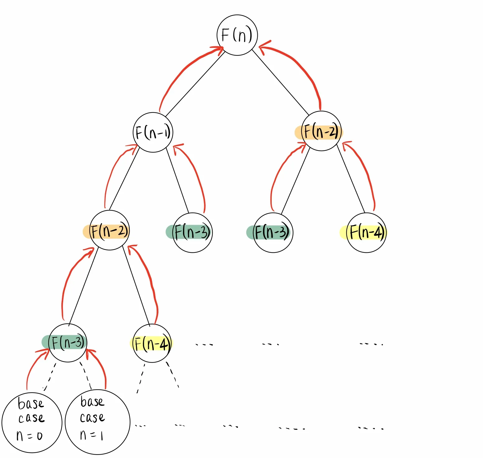
Top-down dynamic programming

To save time, we can reuse the solutions to repeated subproblems. Top-down dynamic programming is a kind of dynamic programming that augments the multiple recursion algorithm with a data structure to store or cache the result of each subproblem. Recursion is only used to solve each unique subproblem exactly once, leading to a linear time algorithm for computing the N^th Fibonacci number.

private static long[] F = new long[92];

public static long fib(int N) {
    if (N == 0 || N == 1) {
        return N;
    }
    if (F[N] == 0) {
        F[N] = fib(N - 1) + fib(N - 2);
    }
    return F[N];
}

Top-down dynamic programming is also known as memoization because it provides a way to turn multiple recursion with repeated subproblems into dynamic programming by remembering past results.

The data structure needs to map each input to its respective result. In the case of fib, the input is an int and the result is a long. Because the integers can be directly used as indices into an array, we chose to use a long[] as the data structure for caching results. But, in other programs, we may instead want to use some other kind of data structure like a Map to keep track of each input and result.

Bottom-up dynamic programming

Like top-down dynamic programming, bottom-up dynamic programming is another kind of dynamic programming that also uses the same data structure to store results. But bottom-up dynamic programming populates the data structure using iteration rather than recursion, requiring the algorithm designer to carefully order computations.

public static long fib(int N) {
    long[] F = new long[N + 1];
    F[0] = 0;
    F[1] = 1;
    for (int i = 2; i <= N; i += 1) {
        F[i] = F[i - 1] + F[i - 2];
    }
    return F[N];
}

After learning both top-down and bottom-up dynamic programming, we can see that there’s a common property between the two approaches.

Dynamic programmming

An algorithm design paradigm for speeding-up algorithms that makes multiple recursive calls by identifying and reusing solutions to repeated recursive subproblems.

Disjoint Sets

1. Trace Kruskal’s algorithm to find a minimum spanning tree in a graph.
2. Compare Kruskal’s algorithm runtime on different disjoint sets implementations.
3. Describe opportunities to improve algorithm efficiency by identifying bottlenecks.

A few weeks ago, we learned Prim’s algorithm for finding a minimum spanning tree in a graph. Prim’s uses the same overall graph algorithm design pattern as breadth-first search (BFS) and Dijkstra’s algorithm. All three algorithms:

• use a queue or a priority queue to determine the next vertex to visit,
• finish when all the reachable vertices have been visited,
• and depend on a neighbors method to gradually explore the graph vertex-by-vertex.

Even depth-first search (DFS) relies on the same pattern. Instead of iterating over a queue or a priority queue, DFS uses recursive calls to determine the next vertex to visit. But not all graph algorithms share this same pattern. In this lesson, we’ll explore an example of a graph algorithm that works in an entirely different fashion.

Kruskal’s algorithm

Kruskal’s algorithm is another algorithm for finding a minimum spanning tree (MST) in a graph. Kruskal’s algorithm has just a few simple steps:

1. Given a list of the edges in a graph, sort the list of edges by their edge weights.
2. Build up a minimum spanning tree by considering each edge from least weight to greatest weight.
3. Check if adding the current edge would introduce a cycle.
4. If it doesn’t introduce a cycle, add it! Otherwise, skip the current edge and try the next one.

The algorithm is done when |V| - 1 edges have been added to the growing MST. This is because a spanning tree connecting |V| vertices needs exactly |V| - 1 undirected edges.

You can think of Kruskal’s algorithm as another way of repeatedly applying the cut property.

Prim’s algorithm

Applied the cut property by selecting the minimum-weight crossing edge on the cut between the visited vertices and the unvisited vertices. In each iteration of Prim’s algorithm, we chose the next-smallest weight edge to an unvisited vertex. Since we keep track of a set of visited vertices, Prim’s algorithm never introduces a cycle.

Kruskal’s algorithm

Instead of growing the MST outward from a single start vertex, there are lots of small independent connected components, or disjoint (non-overlapping) sets of vertices that are connected to each other.

Informally, you can think of each connected component as its own “island”. Initially, each vertex is its own island. These independent islands are gradually connected to neighboring islands by choosing the next-smallest weight edge that doesn’t introduce a cycle.¹

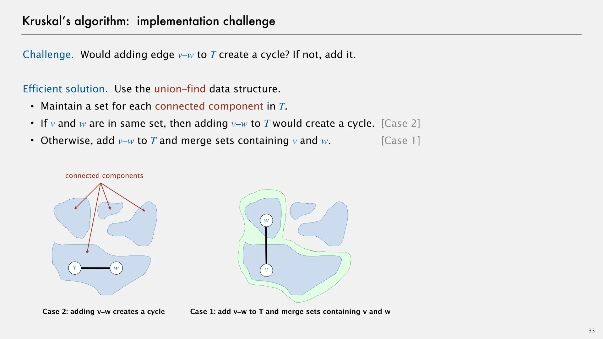
In case 2 (on the left of the above slide), adding an edge v-w creates a cycle within a connected component. In case 1 (on the right of the above slide), adding an edge v-w merges two connected components, forming a larger connected component.

Disjoint sets abstract data type

The disjoint sets (aka union-find) abstract data type is used to maintain the state of connected components. Specifically, our disjoint sets data type stores all the vertices in a graph as elements. A Java interface for disjoint sets might include two methods.

find(v)

Returns the representative for the given vertex. In Kruskal’s algorithm, we only add the current edge to the result if find(v) != find(w).

union(v, w)

Connects the two vertices v and w. In Kruskal’s algorithm, we use this to keep track of the fact that we joined the two connected components.

Using this DisjointSets data type, we can now implement Kruskal’s algorithm.

kruskalMST(Graph<V> graph) {
    // Create a DisjointSets implementation storing all vertices
    DisjointSets<V> components = new DisjointSetsImpl<V>(graph.vertices());
    // Get the list of edges in the graph
    List<Edge<V>> edges = graph.edges();
    // Sort the list of edges by weight
    edges.sort(Double.comparingDouble(Edge::weight));

    List<Edge<V>> result = new ArrayList<>();
    int i = 0;
    while (result.size() < graph.vertices().size() - 1) {
        Edge<V> e = edges.get(i);
        if (!components.find(e.from).equals(components.find(e.to))) {
            components.union(e.from, e.to);
            result.add(e);
        }
        i += 1;
    }
    return result;
}

The remainder of this lesson will focus on how we can go about implementing disjoint sets.

Look-over the following slides where Robert Sedgewick and Kevin Wayne introduce 3 ways of implementing the disjoint sets (union-find) abstract data type.

Union-Find data structures

Quick-find

Optimizes for the find operation.

Quick-union

Optimizes for the union operation, but doesn’t really succeed.

Weighted quick-union

Addresses the worst-case height problem introduced in quick-union.