Graphs

Graph data types, traversals, and MSTs.

1. Graph Data Type
   1. Husky Maps
   2. Vertices and edges
   3. Undirected graph abstract data type
   4. Directed graph abstract data type
   5. Adjacency lists data structure
2. Graph Traversals
   1. Problems and solutions

Graph Data Type

Graph.javaDigraph.java

1. Identify the features and representation for an example graph or graph problem.
2. Analyze the runtime of a graph representation in terms of vertices and edges.
3. Analyze the affordances of a graph interface or method for a particular problem.

Most of the data structures we’ve seen so far organize elements according to the properties of data in order to implement abstract data types like sets, maps, and priority queues.

• Search trees use the properties of an element to determine where it belongs in the search tree. In TreeSet and TreeMap, the ordering relation is defined by the key’s compareTo.
• Binary heaps compare the given priority values to determine whether to sink or swim a node in the heap. In PriorityQueue, the priority values are also defined by the key’s compareTo.
• Hash tables use the properties of an element to compute a hash value, which then determines the bucket index. In HashSet and HashMap, the hash function is defined by the key’s hashCode.

All these data structures rely on properties of data to achieve efficiency. Checking if an element is stored in a balanced search tree containing 1 billion elements only requires about 30 comparisons—which sure beats having to check all 1 billion elements in an unsorted array. This is only possible because (1) the compareTo method defines an ordering relation and (2) the balanced search tree maintains log N height for any assortment of N elements.

But if we step back, all of this happens within the internal implementation details of the balanced search tree. Clients or other users of a balanced search tree treat it as an abstraction, or a structure that they can use without knowing its implementation details. In fact, the client can’t assume any particular implementation because they’re writing their code against more general interfaces like Set, Map, or Autocomplete.

Graphs, however, represent a totally different kind of abstract data type with different goals. Rather than focus on enabling efficient access to data, graphs focus on representing client-defined relationships between data.

Although graphs may look like weirdly-shaped trees, they are used in very different situations. The greatest difference lies in how a graph is used by a client. Instead of only specifying the element to add in a graph, we often will also specify the edges or relationships between elements too. Much of the usefulness of a graph comes from the explicit relationships between elements.

Husky Maps

In the Husky Maps case study, the MapGraph class represents all the streets in the Husky Maps app. Let’s focus on how data is represented in a graph.

public class MapGraph {
    private final Map<Point, List<Edge<Point>>> neighbors;
}

Here’s a breakdown of the data type for the neighbors variable:

Map<Point, List<Edge<Point>>>

A map where the keys are unique Point objects, and the values are the “neighbors” of each Point.

Point

An object that has an x coordinate and a y coordinate. Each point can represent a physical place in the real world, like a street intersection.

List<Edge<Point>>

A list of edges to other points. Each key is associated with one list of values; in other words, each Point is associated with a list of neighboring points.

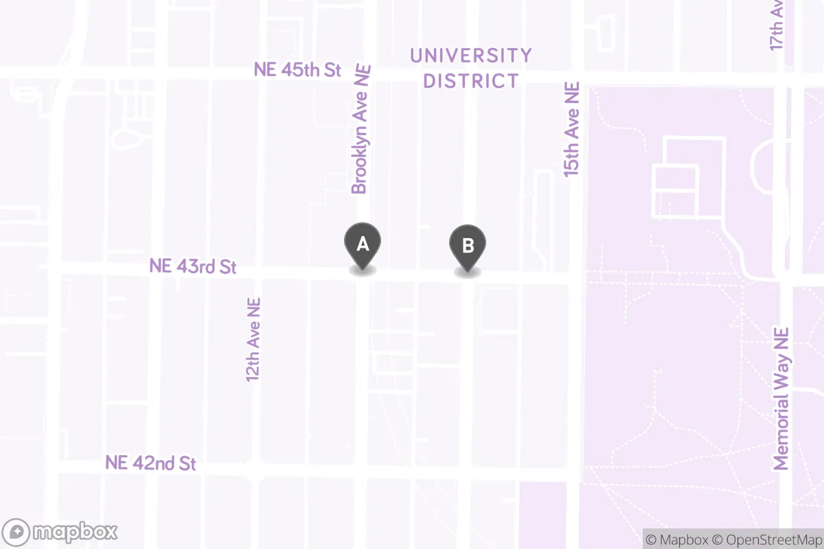
In this image, the Point labeled A represents the intersection Brooklyn Ave NE & NE 43rd St while the Point labeled B represents the intersection University Way NE & NE 43rd St. We say that the two points are “neighbors” because there’s a stretch of NE 43rd St in front of the light rail station that directly connects the two points.

More generally, a graph is a data type composed of vertices and edges defined by the client. In Husky Maps, the vertices are unique Point objects while the edges are stretches of road connecting points. Street intersections are connected to other street intersections. Unlike lists, deques, sets, maps, and priority queues that are defined largely by how they organize elements, graphs are defined by vertices and edges that define relationships between vertices.

In MapGraph, we included an edge representing the stretch of NE 43rd St in front of the light rail station. But this stretch of road is only accessible to buses, cyclists, and pedestrians. Personal vehicles are not allowed on this stretch of road, so the inclusion of this edge suggests that this graph would afford applications that emphasize public transit, bicycling, or walking. Graph designers make key decisions about what data is included and represented in their graph, and these decisions affect what kinds of problems can be solved.

Vertices and edges

Vertex (node)

A basic element of a graph.

In MapGraph, vertices are represented using the Point class.

Edge

A direct connection between two vertices v and w in a graph, usually written as (v, w). Optionally, each edge can have an associated weight.

In MapGraph, edges are represented using the Edge class. The weight of an edge represents the physical distance between the two points adjacent to the edge.

Given a vertex, its edges lead to neighboring (or adjacent) vertices. In this course, we will always assume two restrictions on edges in a graph.

• No self-loops. A vertex v cannot have an edge (v, v) back to itself.
• No parallel (duplicate) edges. There can only exist at most one edge (v, w).

There are two types of edges.

Undirected edges

Represent pairwise connections between vertices allowing movement in both directions. Visualized as lines connecting two vertices.

In MapGraph, undirected edges are like two-way streets where traffic can go in both directions.

Directed edges

Represent pairwise connections between vertices allowing movement in a single direction. Visualized as arrows connecting one vertex to another.

In MapGraph, directed edges are like one-way streets.

Undirected graph abstract data type

An undirected graph (or simply “graph” without any qualifiers) is an abstract data type that contains zero or more vertices and zero or more undirected edges between pairs of vertices. The following slide¹ describes some undirected graph terminology.

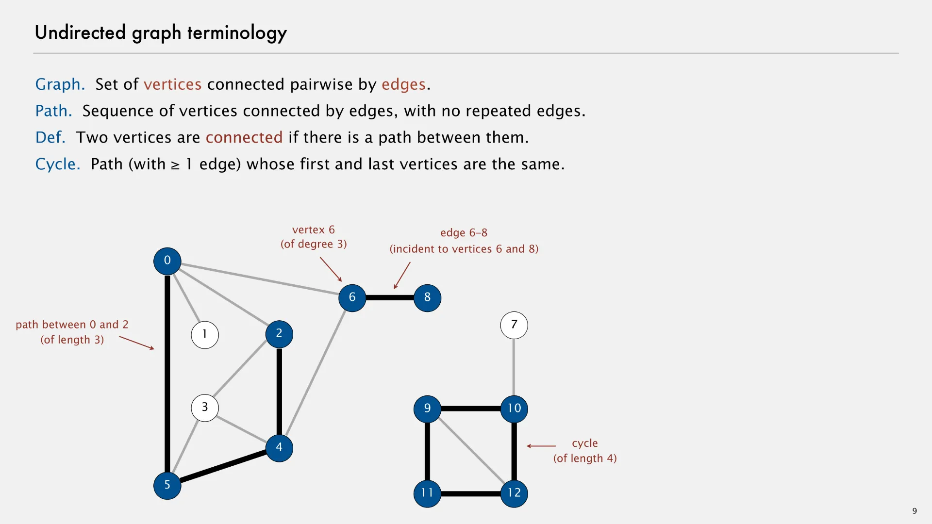
Path

Sequence of vertices connected by undirected edges, with no repeated edges.

Two vertices are connected if there is a path between them.

Cycle

Path (with 1 or more edges) whose first and last vertices are the same.

Degree

Number of undirected edges associated with a given vertex.

An interface for an undirected graph could require an addEdge and neighbors method.

public interface UndirectedGraph<V> {

    /** Add an undirected edge between vertices (v, w). */
    public void addEdge(V v, V w);

    /** Returns a list of the edges adjacent to the given vertex. */
    public List<Edge<V>> neighbors(V v);
}

Directed graph abstract data type

A directed graph (or “digraph”) is an abstract data type that contains zero or more vertices and zero or more directed edges between pairs of vertices. The following slide¹ describes some directed graph terminology.

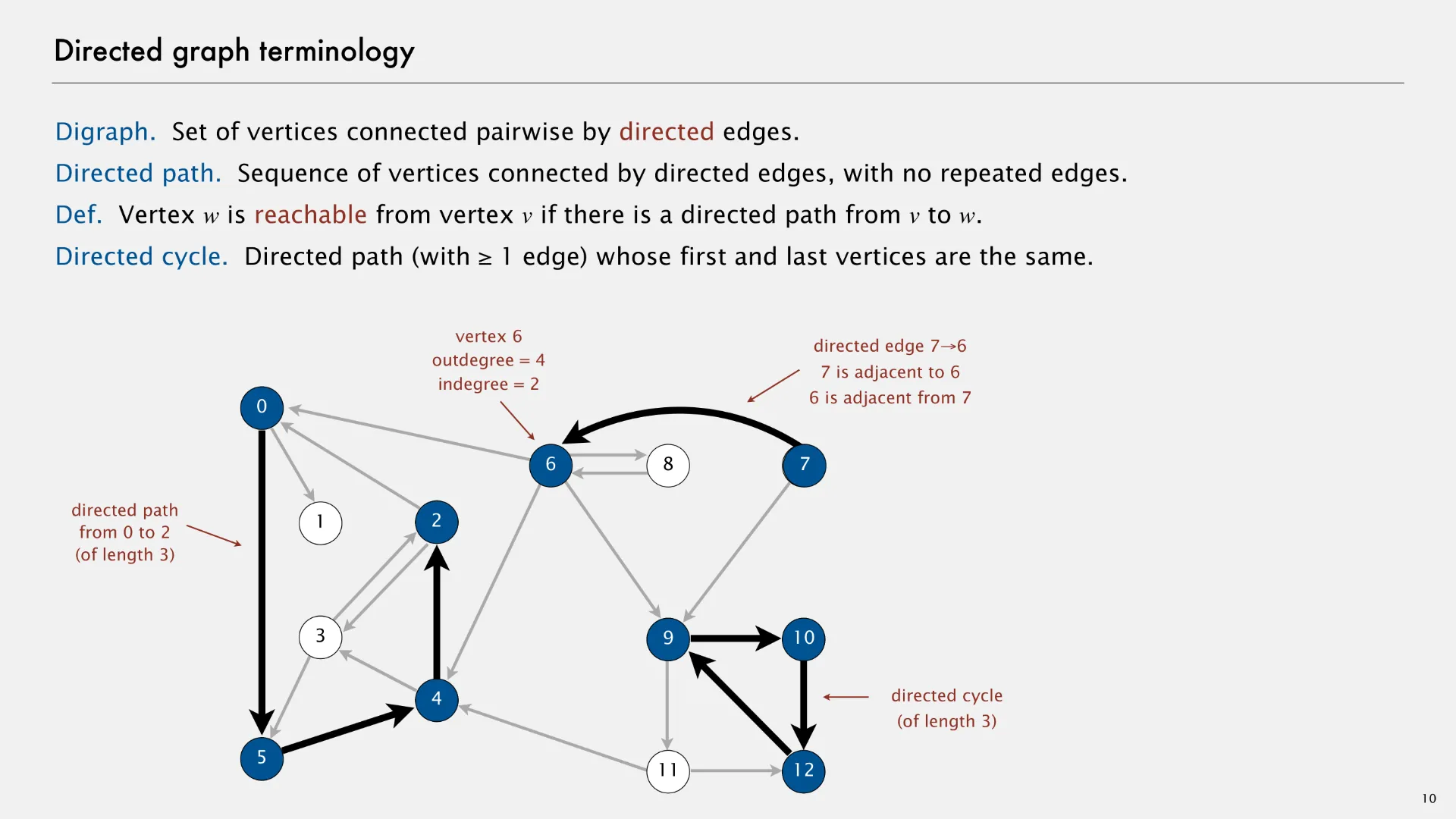
Although parallel (duplicate) edges are not allowed, a directed graph can have edges in both directions between each pair of nodes. In the example above, note there are edges (2, 3) and (3, 2), as well as edges (6, 8) and (8, 6). These two pairs of edges allow for movement in both directions.

Directed path

Sequence of vertices connected by directed edges, with no repeated edges.

Vertex w is reachable from vertex v if there is a directed path from v to w.

Directed cycle

Directed path (with 1 or more edges) whose first and last vertices are the same.

Outdegree

Number of directed edges outgoing from a given vertex.

Indegree

Number of directed edges incoming to the given vertex.

An interface for an directed graph could also require an addEdge and neighbors method, just as in the undirected graph example.

public interface DirectedGraph<V> {

    /** Add an directed edge between vertices (v, w). */
    public void addEdge(V v, V w);

    /** Returns a list of the outgoing edges from the given vertex. */
    public List<Edge<V>> neighbors(V v);
}

Adjacency lists data structure

Adjacency lists is a data structure for implementing both undirected graphs and directed graphs.

Adjacency lists

A graph data structure that associates each vertex with a list of edges.

MapGraph uses an adjacency lists data structure: the neighbors map associates each Point with a List<Edge<Point>>. The adjacency lists provides a very direct implementation of the DirectedGraph interface methods like addEdge and neighbors.

public class MapGraph implements DirectedGraph<Point> {
    private final Map<Point, List<Edge<Point>>> neighbors;

    /** Constructs a new map graph. */
    public MapGraph(...) {
        neighbors = new HashMap<>();
    }

    /** Adds a directed edge to this graph using distance as weight. */
    public void addEdge(Point from, Point to) {
        if (!neighbors.containsKey(from)) {
            neighbors.put(from, new ArrayList<>());
        }
        neighbors.get(from).add(new Edge<>(from, to, estimatedDistance(from, to)));
    }

    /** Returns a list of the outgoing edges from the given vertex. */
    public List<Edge<Point>> neighbors(Point point) {
        if (!neighbors.containsKey(point)) {
            return new ArrayList<>();
        }
        return neighbors.get(point);
    }
}

The MapGraph class doesn’t have a method for adding just a single vertex or getting a list of all the vertices or all the edges. These aren’t necessary for Husky Maps. But in other situations, you might like having these methods that provide different functionality. The Java developers did not provide a standard Graph interface like they did for List, Set, or Map because graphs are often custom-designed for specific problems. What works for Husky Maps might not work well for other graph problems.

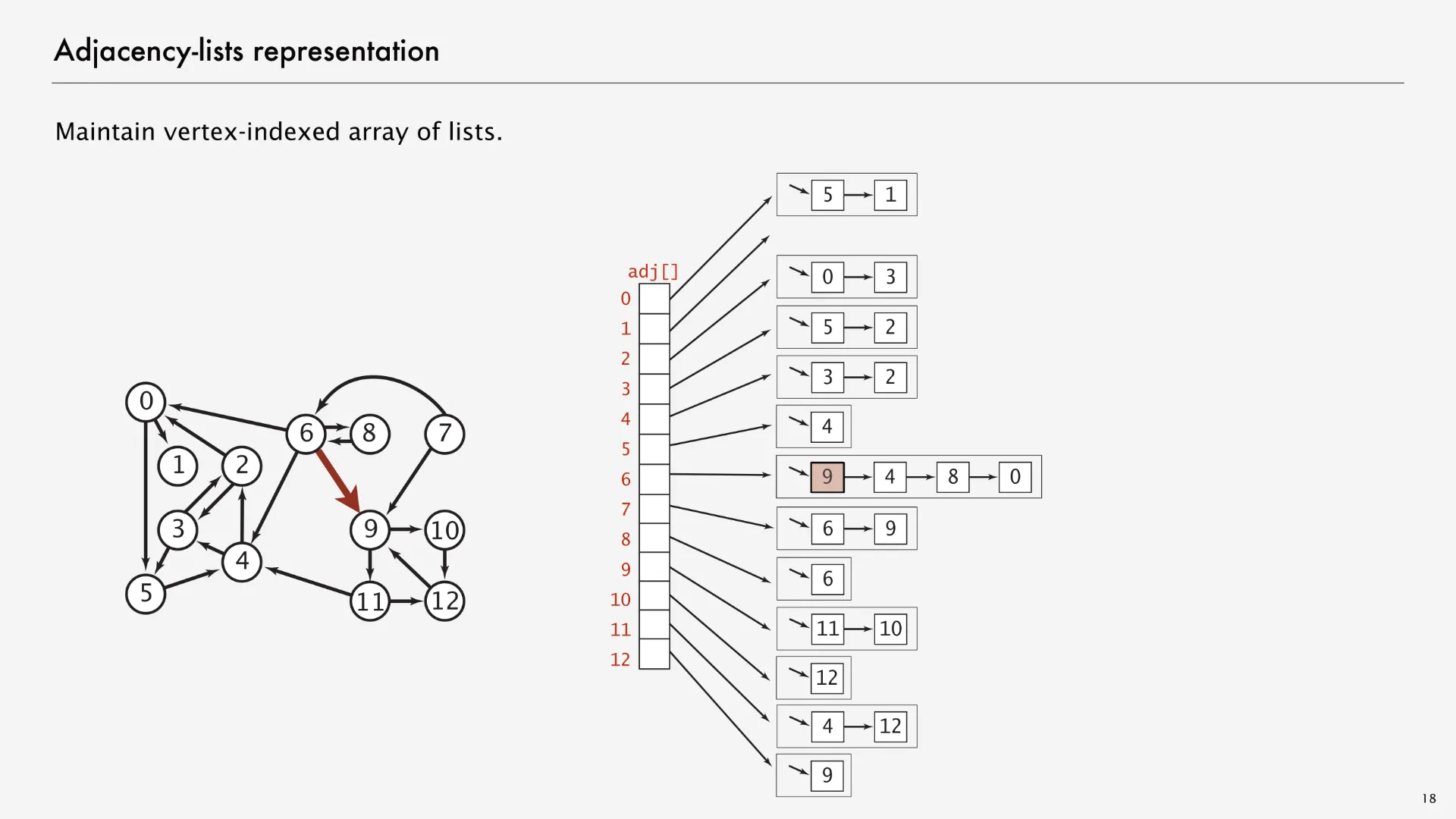
There are many options for Map and Set implementations. Instead of HashMap, we could have chosen TreeMap; instead of HashSet, TreeSet. However, we’ll often visualize adjacency lists by drawing the map as an array associating each vertex with a linked list representing its neighbors. The following graph visualization¹ on the left matches with the data structure visualization on the right, with the edge (6, 9) marked red in both the left and the right side.

Adjacency lists aren’t the only way to implement graphs. Two other common approaches are adjacency matrices and edge sets. Both of these approaches provide different affordances (making some graph methods easier to implement or more efficient in runtime), but adjacency lists are still the most popular option for the graph algorithms we’ll see in this class. Keith Schwarz writes on StackOverflow about a few graph problems where you might prefer using an adjacency matrix over an adjacency list but summarizes at the top:

Adjacency lists are generally faster than adjacency matrices in algorithms in which the key operation performed per node is “iterate over all the nodes adjacent to this node.” That can be done in time O(deg(v)) time for an adjacency list, where deg(v) is the degree of node v, while it takes time Θ(n) in an adjacency matrix. Similarly, adjacency lists make it fast to iterate over all of the edges in a graph—it takes time O(m + n) to do so, compared with time Θ(n²) for adjacency matrices.

Some of the most-commonly-used graph algorithms (BFS, DFS, Dijkstra’s algorithm, A* search, Kruskal’s algorithm, Prim’s algorithm, Bellman-Ford, Karger’s algorithm, etc.) require fast iteration over all edges or the edges incident to particular nodes, so they work best with adjacency lists.

Graph Traversals

BreadthFirstPaths.javaDepthFirstPaths.java

1. Trace and explain each data structure in BFS and DFS graph traversal.
2. Analyze the runtime of a graph algorithm in terms of vertices and edges.
3. Define an appropriate graph abstraction for a given image processing problem.

How do we use a graph to solve problems like computing navigation directions? Before we can discuss graph algorithms, we’ll need a way to traverse a graph or explore all of its data. To traverse a tree, we can start from the overall root and recursively work our way down. To traverse a hash table, we can start from bucket index 0 and iterate over all the separate chains. But for a graph, where do we start the traversal?

By applying the recursive tree traversal idea, we discovered a graph algorithm called depth-first search (DFS). Depth-first search isn’t the only graph traversal algorithm, and it’s often compared to another graph traversal algorithm called breadth-first search (BFS). BFS will be the template for many of the graph algorithms that we’ll learn in the coming lessons.

Breadth-first search (BFS)

An iterative graph traversal algorithm that expands outward, level-by-level, from a given start vertex.

void bfs(Graph<V> graph, V start) {
    Queue<V> perimeter = new ArrayDeque<>();
    Set<V> visited = new HashSet<>();

    perimeter.add(start);
    visited.add(start);

    while (!perimeter.isEmpty()) {
        V from = perimeter.remove();
        // Process the current vertex by printing it out
        System.out.println(from);

        for (Edge<V> edge : graph.neighbors(from)) {
            V to = edge.to;
            if (!visited.contains(to)) {
                perimeter.add(to);
                visited.add(to);
            }
        }
    }
}

Depth-first search (DFS)

A recursive graph traversal algorithm that explores as far as possible from a given start vertex until it reaches a base case and needs to backtrack.

void dfs(Graph<V> graph, V start) {
    dfs(graph, start, new HashSet<>());
}

dfs(Graph<V> graph, V from, Set<V> visited) {
    // Process the current vertex by printing it out
    System.out.println(from);
    visited.add(from);

    for (Edge<V> edge : graph.neighbors(from)) {
        V to = edge.to;
        if (!visited.contains(to)) {
            dfs(graph, to);
        }
    }
}

BFS and DFS represent two ways of traversing over all the data in a graph by visiting all the vertices and checking all the edges. BFS and DFS are like the for loops of graphs: on their own, they don’t solve a specific problem, but they are an important building block for graph algorithms.

BFS provides a lot more utility than DFS in this context because it can be used to find the shortest paths in a unweighted graph with the help of two extra data structures called edgeTo and distTo.

• Map<V, Edge<V>> edgeTo maps each vertex to the edge used to reach it in the BFS traversal.
• Map<V, Integer> distTo maps each vertex to the number of edges from the start vertex.

We’ll study these two maps in greater detail over the following lessons.

Problems and solutions

Whereas sets, maps, and priority queues emphasize efficient access to elements, graphs emphasize not only elements (vertices) but also the relationships between elements (edges). The efficiency of a graph data structure depends on the underlying data structures used to represent its vertices and edges. But there’s another way to understand graphs through the lens of computational problems and algorithmic solutions.

Computational problem

An abstract problem that can be represented, formalized, and/or solved using algorithms.

In Java, we often represent problems using interfaces describing expected functionality.

Sorting is the problem of rearranging elements according to an ordering relation (via comparison). Sets are an example of an abstract data type that represents a collection of unique elements. Graph traversal is the problem of visiting/checking/processing each vertex in a graph.

Algorithmic solution

A a sequence of steps or description of process that can be used to solve computational problems.

In Java, we often represent solutions using classes detailing how to implement functionality.

Insertion sort, selection sort, and merge sort are algorithms for sorting. Search trees and hash tables are algorithms for implementing sets. BFS and DFS are algorithms for graph traversal.

This relationships suggests that problems like graph search can be represented using interfaces, which are then implemented by solutions that are represented using classes. In Husky Maps, the graphs.shortestpaths package includes interfaces and classes for finding the shortest paths in a directed graph.

public interface ShortestPathSolver<V>
public class DijkstraSolver<V> implements ShortestPathSolver<V>
public class BellmanFordSolver<V> implements ShortestPathSolver<V>
public class ToposortDAGSolver<V> implements ShortestPathSolver<V>

Each of these graph algorithms—Dijkstra’s algorithm, Bellman-Ford algorithm, and the toposort-DAG algorithm—do most of their work in the class constructor. If we wanted to add a BFS algorithm to this list, it would take the bfs method defined above and do most of the work inside of the constructor.

public class BreadthFirstSearch<V> {
    private final Map<V, Edge<V>> edgeTo;
    private final Map<V, Integer> distTo;

    public BreadthFirstSearch(Graph<V> graph, V start) {
        edgeTo = new HashMap<>();
        distTo = new HashMap<>();
        Queue<V> perimeter = new ArrayDeque<>();
        Set<V> visited = new HashSet<>();
        perimeter.add(start);
        visited.add(start);
        edgeTo.put(start, null);
        distTo.put(start, 0);
        while (!perimeter.isEmpty()) {
            V from = perimeter.remove();
            for (Edge<V> edge : graph.neighbors(from)) {
                V to = edge.to;
                if (!visited.contains(to)) {
                    edgeTo.put(to, edge);
                    distTo.put(to, distTo.get(from) + 1);
                    perimeter.add(to);
                    visited.add(to);
                }
            }
        }
    }

    /** Returns the unweighted shortest path from the start to the goal. */
    public List<V> solution(V goal) {
        List<V> path = new ArrayList<>();
        V curr = goal;
        path.add(curr);
        while (edgeTo.get(curr) != null) {
            curr = edgeTo.get(curr).from;
            path.add(curr);
        }
        Collections.reverse(path);
        return path;
    }
}

The solution method begins at goal and uses edgeTo to trace the path back to start.

There are hundreds of problems and algorithms for solving them. The field of graph theory investigates these graph problems and graph algorithms.