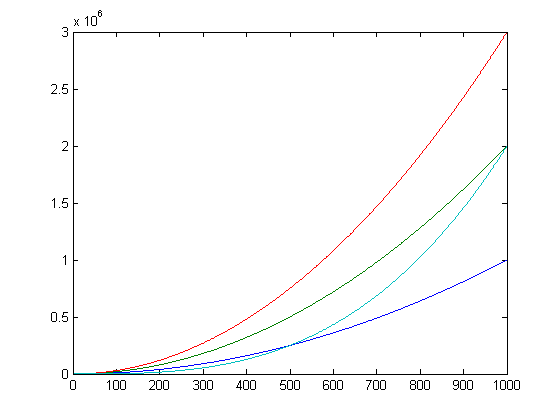
x=[1:1000]; plot(x,x.^2,x,2*x.^2,x,3*x.^2,x,.002*x.^3)
plot of x^2 (blue), 2*x^2 (green), 3*x^2(red), .002*x^3(cyan)
It can be tricky to tell the order of magnitudes of each of the functions.
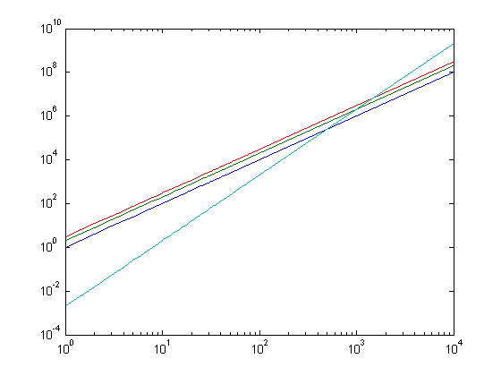
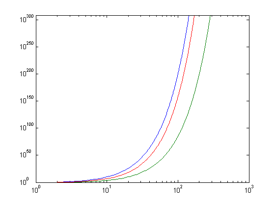
x=[1:10000]; loglog(x,x.^2,x,2*x.^2,x,3*x.^2,x,.002*x.^3)
logplot of x^2 (blue), 2*x^2 (green), 3*x^2(red), .002*x^3(cyan)
But as a log-log plot, the trend becomes apparent. Each of the quadratics have
a slope of 2, just translated differently, whereas the cubic has a slope of 3.
What do these slopes mean? A slope of two means doubling the problem
size quadruples the running time. A slope of three means doubling results
in an 8x increase.
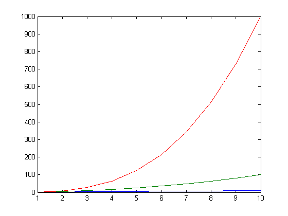
x=[1:10];plot(x,x,x,x.^2,x,x.^3)
Clearly the cubic (red) grows much faster than the quadratic (green), and way way faster than the linear (blue).
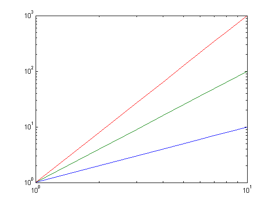
x=[1:10];loglog(x,x,x,x.^2,x,x.^3)
In a loglog plot, it becomes easier to capture such wide magnitudes in the same plot.
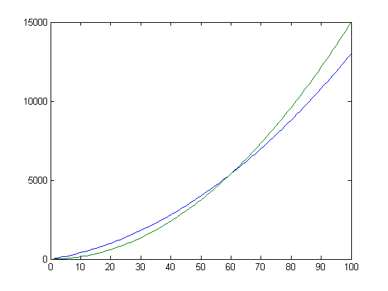
x=[1:100];plot(x,x.^2+30*x,x,1.5*x.^2)
plot of x^2+30x (blue), 1.5*x^2 (green)
Note that after some point, the green function becomes larger, showing that x^2+30x is O(x^2)
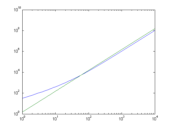
x=[1:10000];loglog(x,x.^2+30*x,x,1.5*x.^2)
loglog plot of x^2+30x (blue), 1.5*x^2 (green)
In the loglog plot, we can see that after some point, the lower-order terms stop dominating, and the
slope of the function is 2. Remember that translating it up or down is equivalent to a constant scale.
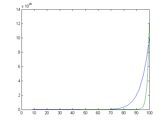
x=[1:100];plot(x,x.^15,x,2.^x)
As fast as x^15 (blue) grows, 2^x (green) grows even faster.
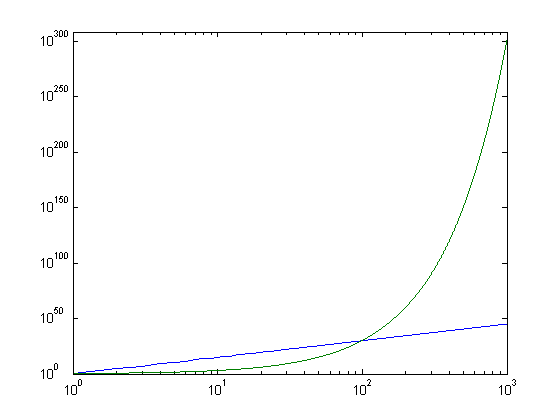
x=[1:1000];loglog(x,x.^15,x,2.^x)
The difference in growth between a polynomial and an exponential becomes ever clearer.
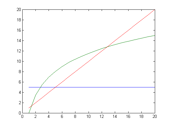
x=[1:20];plot(x,0*x+5,x,5*log(x),x,x)
5 (blue), 5 log x (green), x (red)
Note that over time, 5 log x performs better than x, but can never compete with constant time.
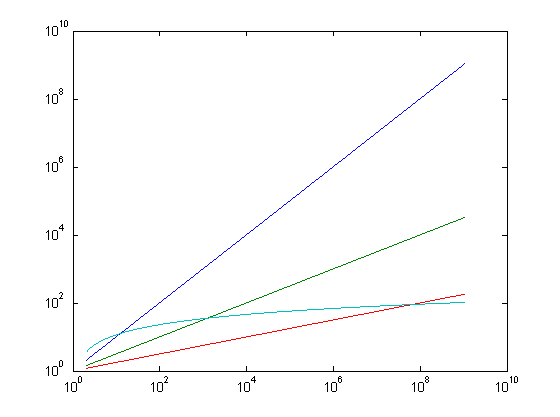
y=[1:.01:30];x=2.^y;loglog(x,x,x,x.^.5,x,x.^.25,x,5*log(x))
x (blue), x^.5 (green), x^.25 (red), 5 log(x) (cyan)
On a loglog plot, the slope of log(x) tends to zero as x gets very large.
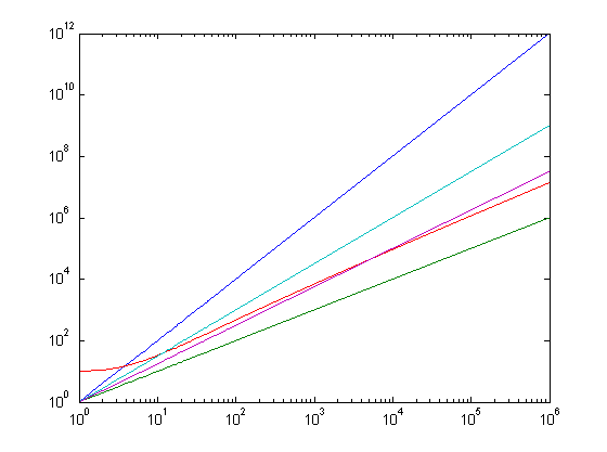
x=[1:1000000];loglog(x,x.*x,x,x,x,x.*log(x)+10,x,x.^1.5,x,x.^1.25)
x log x + 10 (red), x^2 (blue), x^1.5 (cyan), x^1.25 (magenta), x (green)
Note how n log n is O(n^2), O(n^1.5), O(n^1.25), O(n^(1+epsilon)), but not
O(n).
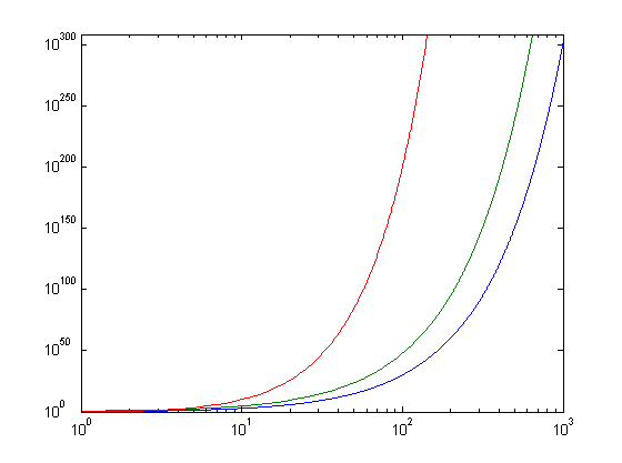
x=[1:1000];loglog(x,2.^x,x,3.^x,x,x.^x)
2^x (blue), 3^x (green), x^x (red)
As fast as 2^x and 3^x grow, x^x is even faster.
x=[2:1000];loglog(x,x.^x,x,(x/2).^(x/2),x,factorial(x))
x^x (blue), (x/2)^(x/2) (green), x! (red)
This shows the cool bounding that is used for the n log n comparison proof.
There are n! permutations of an n-element list, and any binary tree with
n! leaves must have a minimum depth of log(n!), which is n log n.