This page is from a previous offering of the course. It has been left up for archival purposes.
In this section we will discuss a method for performing running time analysis of recursive algorithms. To summarize the approach, here’s what we’ll do:
- A running time analysis of an algorithm is a function. For our recursive algorithm, we’ll identify a recursive running time function. Such a function is called a recurrence relation.
- Next we will
solve
the recurrence relation, which in our case means converting it into an asymptotically equivalent non-recursive function.
For step 2 of this process, there are many ways to do this. We’ll focus on just one way in the course. We’ll use a method called the tree method.
1 Identifying A Recurrence
First, let’s see how we can express the running time of an algorithm as a recurrence relation. Any recursive algorithm is going to have the following parts:
- Base case: Check if the input is small enough (\leq some constant) to constitute a base case, if so then solve it using an iterative (i.e. non-recursive) approach
- Prepare for recursion: Perform iterative steps of computation in preparation for recursive calls
- Recursive calls: Invoke the algorithm recursively on one or more smaller inputs
- Use recursive results: Perform iterative steps of computation using the results from the recursive calls
We can then apply our standard running time analysis process to these steps as follows:
- We can recognize that the base case does not occur in every recursive invocation, and when it does happen its running time is always constant (base case size must be a constant, and any procedure run on a constant-sized input takes only constant time).
- The remaining three steps all happen sequentially for one another, so we can add together their running times.
- The recursive invocations are just like invoking another function, so we want to use the running time of that function in that place.
Therefore, if we use T(n) to represent the running time of our algorithm, our analysis of the generic recursive procedure above will look something like:
- Base case: Let the constant k be the base case size. If n\leq k then the running time is the constant c. So T(k)=c
- Prepare for recursion: This code is iterative, so we can use our standard process for running time analysis. Call the resulting running time function p(n).
- Recursive calls: Each recursive call will happen on a smaller input. If we want to recurse on inputs of size x_1, x_2, …, x_a then we can write the running time of this portion as T(x_1)+T(x_2)+...+T(x_a).
- Use recursive results: Again, this is iterative, so we can use our standard process. Call the resulting running time function r(n).
All together, we therefore get the following running time:
T(n)=p(n)+T(x_1)+T(x_2)+...+T(x_a)+r(n) where T(k)=c.
This is now a recursive running time function for our algorithm, i.e. a recurrence relation.
For most algorithms each of x_1, x_2, ..., x_a will be of the same size. If we call this x then our recurrence could be expressed as :
T(n)=p(n) + aT(x) + r(n) where T(k)=c.
Furthermore, we can introduce the function f(n)=p(n)+r(n) to express all of the iterative work being done in one stack frame, giving us:
T(n)=aT(x) + f(n) where T(k)=c.
Finally, for most algorithms the value of x is either going to be some fraction of n (called a divide and conquer
pattern) or it will be a constant reduction in size (called a chip and conquer
pattern), and so our recurrence would be one of the following:
- Divide and Conquer: T(n)=aT(\frac{n}{b}) + f(n) where T(k)=c.
- Chip and Conquer: T(n)=aT(n-b) + f(n) where T(k)=c.
In this class nearly all of our recurrence relations will take one of these two shapes, so we’ll focus on that going forward.
1.1 Divide and Conquer Example
Now let’s see an example of this process being applied to a recursive algorithm. Consider the following algorithm which finds the sum of all elements in a list recursively:
public int sum(int[] list){
          return sum_helper(list, 0, list.size);
      }
      private int sum_helper(int[] list, int low, int high){
          if (low == high){ return 0; }
          if (low == high-1){ return list[low]; }
          int middle = (high+low)/2;
          return sum_helper(list, low, middle) + sum_helper(list, middle, high);
      }
For this algorithm, each stack frame is responsible for summing the values in the list between the index low (inclusive) and high (exclusive). If the distance between low and high is 0 then there are no elements in that region, so it returns 0. If the distance between low and high is 1 then there is exactly one element in that region, so it returns that element. Otherwise it divides the region in half, recursively sums the two halves, and adds those results together.
For this algorithm our input size will be measured by the distance between low and high (it is initially n, as that is the size of the original list). The operations we’ll count are additions between elements of the list.
Let’s now assign each step of this algorithm to our generic pattern above:
- Base case: When the input is size 0 or 1, in either case there are no additions being done, so T(1)=T(0)=0.
- Prepare for recursion: For this step we calculate the index that is half way between low and high, there are no additions done among elements of the list here, so p(n)=0.
- Recursive calls: There are two recursive calls, each one on a region half the size of the original, so the running time is T(\frac{n}{2})+T(\frac{n}{2}) or 2T(\frac{n}{2}).
- Use recursive results: This one happens to be on the same line as the recursive calls. This is the step of adding together the results of the recursive calls. This is now an addition between elements of the list, so r(n)=1.
Overall this gives us the recurrence relation:
T(n)=2T(\frac{n}{2}) + 1 where T(1)=T(0)=0. Note that this follows our divide and conquer pattern!
1.2 Chip and Conquer Example
Next we consider this recursive algorithm, which also sums a list recursively:
public int sum(int[] list){
          return sum_helper(list, 0, list.size);
      }
      private int sum_helper(int[] list, int low, int high){
          if (low == high){ return 0; }
          if (low == high-1){ return list[low]; }
          return list[low] + sum_helper(list, low+1, high) ;
      }
As with the previous algorithm, each stack frame is responsible for summing the values in the list between the index low (inclusive) and high (exclusive). If the distance between low and high is 0 then there are no elements in that region, so it returns 0. If the distance between low and high is 1 then there is exactly one element in that region, so it returns that element. The difference here is that instead of dividing the region in half, this algorithm recursively finds the sum of the region excluding the index low, then adds the value at that index to the result.
As before, our input size will be measured by the distance between low and high (it is initially n, as that is the size of the original list). The operations we’ll count are additions between elements of the list.
Let’s now assign each step of this algorithm to our generic pattern above:
- Base case: When the input is size 0 or 1, in either case there are no additions being done, so T(1)=T(0)=0.
- Prepare for recursion: For this step we calculate the index that is half way between low and high, there are no additions done among elements of the list here, so p(n)=0.
- Recursive calls: There is one recursive call, each one on a region one smaller than the original, so the running time is T(n-1).
- Use recursive results: This one happens to be on the same line as the recursive call. This is the step of adding the value at index low to the result of the recursive call. This is now an addition between elements of the list, so r(n)=1.
Overall this gives us the recurrence relation:
T(n)=T(n-1) + 1 where T(1)=T(0)=0. Note that this follows our chip and conquer pattern!
2 Solving Recurrences
Now that we’ve seen how to identify a recursive running time function for our recursive algorithms, let’s wee how we can solve them. Let’s start with our chip an conquer recurrence T(n)=T(n-1)+1.
Our goal is to express this recurrence so that we have an equivalent function (at least asymptotically) that is expressed non-recursively. With that in mind, let’s start by trying to simplify the recurrence.
Ultimately we want to know the value of T(n) in terms of n. Our definition of T(n) tells us that T(n)=T(n-1)+1. We could then reapply the definition of T to identify the value of T(n-1), giving us T(n)=(T(n-2)+1)+1. We can repeat this process over and over again, replacing T(x) with T(x-1)+1:
T(n)=T(n-1)+1=T(n-2)+1+1=T(n-3)+1+1+1=T(n-4)+1+1+1+1+....
This substitution will then repeat until the argument to T is 1, since this is our base case. In the end we therefore get T(n)=T(1)+1+1+1+1+...+1 where we have accumulated a +1 term for each substitution we did until reaching our base case. To find our running time, we just need to figure out the number of substitutions we had to do. Recalling back to the recursive algorithm this came from, this matches the length of the chain of stack frames we have from our original input of size n to our base case of size 1. To identify this number we need to answer the question How many times must we subtract 1 from n until we reach the value 1?
. The answer to this should be the value of i such that n-i=1, and so solving for i we get n-1. This tells us that T(n) through repeated substitution becomes n-1 ones added together, and so our running time is \Theta(n).
2.1 The Tree Method
Next we’ll look at how we can take the repeated substitution
approach and apply a bit more structure to it so that we can use it as a tool for solving more complex recurrence relations. We will call this procedure the Tree Method. Essentially, the tree method works by performing this repeated substitution, but making each substitution (i.e. stackframe in the recursion) a node in a tree.
2.1.1 Chip and Conquer
Let’s start by reexpressing our repeated substitution of T(n)=T(n-1)+1 in this way. The root of our tree will correspond to the stackframe for our original invocation of the algorithm, that in which the input size is n. That stackframe makes one recursive call on an input of size n-1, which makes another recursive call on an input size n-2, which makes another with size n-3, etc. This chain of invocations continues until we reach a base case. As per our discussion earlier, the length of this chain is therefore n-1. All that remains is to identify the total amount of work done within each stackframe, and then add those together. In our recurrences f(n) represents the non-recursive work done in a stackframe with input size n, and in this case f(n)=1. This tells us we need to add 1 for each stackframe in our chain, therefore giving a running time of n-1 = \Theta(n). We call this the tree method
because we’ll see that this chain
of stackframes is actually a tree with no branches. One we analyze our divide and conquer recurrence we’ll see that our tree has branches because each stackframe has multiple recursive calls.
We depict this procedure graphically below:
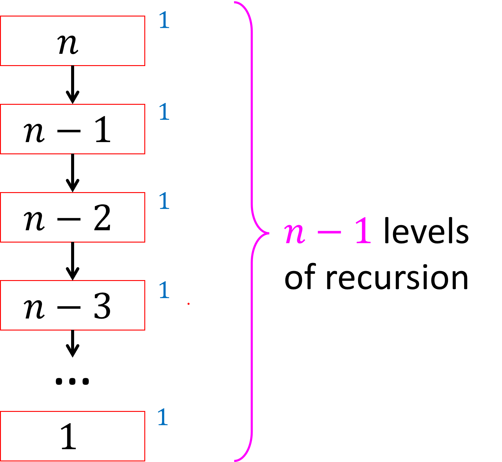
We represent each stackframe as a square, write the input size for that stackframe within the square, and then write the non-recursive work done in that stackframe next to each square. Our objective is to sum together all the values written next to the squares.
The following describes the general process we can use to solve chip and conquer recurrences using the tree method:
To solve a recurrence of the form T(n)=aT(n-b)+f(n):
- Use the recurrence to draw a tree
- a is the branching factor of the tree (e.g. if a=2 then it’s a binary tree)
- Subtract b from the parent’s input size to get each child’s input size
- The height of the tree is \frac{n}{b}.
- Work done per node is given by applying f(n) to that node’s input size, write that value beside each node.
- Add the total work done across all nodes
- Express the work per level i as an expression using i
- Write a series adding the work per level for i=0 through i=\frac{n}{b}.
- Solve the series
- Simplify the sum asymptotically
For reasons we’ll get to later in this reading, It is important that the correct values of a and b are chosen in order to get the right asymptotic running time. It is also important to get the function f(n) asymptotically correct (i.e. you can use any other function g(n) here so long as g(n)=\Theta(f(n)) and get the same result). The exact size and running time of the base cases will never make a difference in an asymptotic analysis.
2.1.2 Divide and Conquer
Now let’s see how we can use our tree method to solve the divide and conquer recurrence T(n)=2T(\frac{n}{2}) + 1 where T(1)=T(0)=0. Let’s use the process from above. As before, we will start with the stackframe where the input is of size n. That stackframe then invokes two recursive calls, each on an input of size \frac{n}{2}. Each of those then also invokes two recursive calls, each on an input of size \frac{n}{4}. This means after two rounds we have seven total stack frames: one root, two at depth 1, and four at depth 2. Overall, each level of the tree will have twice as many nodes as the prior level (each node invokes two recursive calls), and the input size to each will be half the size as those on the prior level. Each stackframe will then do one addition operation.
We can depict this relationship among stackframes like this:
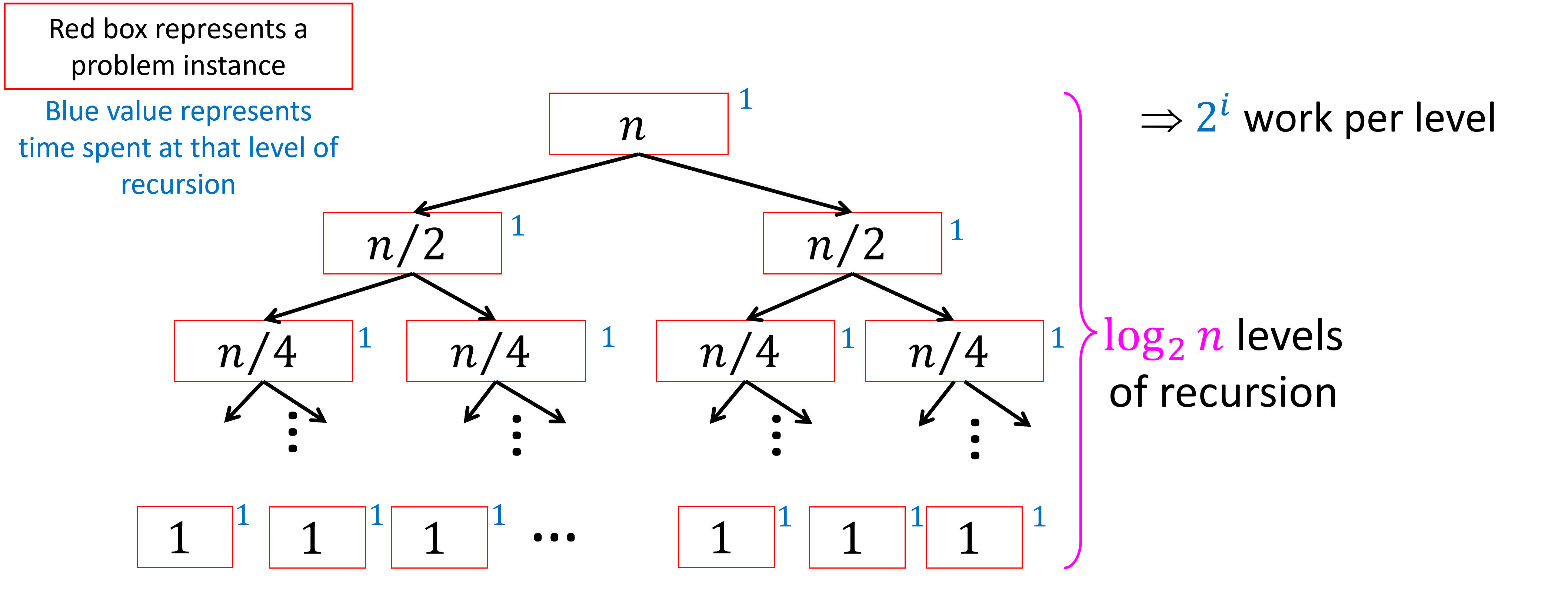
Let’s see why the height of this tree is log_2(n). Similar to the chip-and-conquer recurrence, the height of the tree is determined by the distance from our root to our leaves, because this is the number of times we must shrink our original input of size n before we reach the base case. For this algorithm we shrink our input by cutting it in half, so we need to determine how many times we must cut n in half before we get to the value 1. If we cut n in half i times we will have the value \frac{n}{2^i}. This means that we need to find the value of i such that \frac{n}{2^i}=1. Solving for i we get i=\log_2(n).
Now that we have the structure of our tree, we again need to add the total work done among all of the stackframes, meaning we want to sum together all of the values that we wrote down next to the boxes in the tree. The easiest way to do this is generally to first find the sum per-level, then use that to identify a pattern to express the work done at each level i as a function involving i. Then we can write a series summing the work-per-level for i=0 up to i=log_2(n).
For this tree, the amount of work done on level i is equal to the number of nodes in that level. Since we double at each level, the number of nodes on level i is 2^i. This means our running time should be the solution to the series \sum_{i=0}^{\log_2 n} 2^i. Using our geometric series formula, this is \frac{2^{\log_2 n}-1}{2-1}=n. Therefore the running time is \Theta(n).
The following describes the general process we can use to solve divide and conquer recurrences using the tree method:
To solve a recurrence of the form T(n)=aT(\frac{n}{b})+f(n):
- Use the recurrence to draw a tree
- a is the branching factor of the tree (e.g. if a=2 then it’s a binary tree)
- Divide the parent’s input size by b to get each child’s input size
- The height of the tree is \log_b n.
- Work done per node is given by applying f(n) to that node’s input size, write that value beside each node.
- Add the total work done across all nodes
- Express the work per level i as an expression using i
- Write a series adding the work per level for i=0 through i=\log_b n.
- Solve the series
- Simplify the sum asymptotically
3 What’s important
When doing any sort of running time analysis it will be helpful to have an idea of what aspects of your analysis may vs. may not impact your overall asymptotic answer. The following aspects of a recurrence relation do matter (meaning changing them may result in a different asymptotic solution):
- The coefficient on the recursive call. In other words, T_1(n)=a_1T_1(\frac{n}{b})+f(n) might be different from T_2(n)=a_2T_2(\frac{n}{b})+f(n) if a_1\neq a_2.
- The argument to the recursive call. In other words, T_1(n)=aT_1(\frac{n}{b_1})+f(n) might be different from T_2(n)=aT_2(\frac{n}{b_2})+f(n) if b_1\neq b_2.
- The asymptotic behavior of f(n). In other words, T_1(n)=aT_1(\frac{n}{b})+f_1(n) might be different from T_2(n)=aT_2(\frac{n}{b})+f_2(n) if f_1(n) \neq \Theta(f_2(n)).
The following aspects of a recurrence relation do not matter (meaning changing them may result in a different asymptotic solution):
- The constant factors and non-dominant terms of f(n). In other words, T_1(n)=aT_1(\frac{n}{b})+f_1(n) will have the same result as T_2(n)=aT_2(\frac{n}{b})+f_2(n) if f_1(n) = \Theta(f_2(n))
- The size of the base cases. If we evaluate the recurrence using a base case of T(1) vs. a base case of T(2) then the running time will be the same asymptotically.
- The running time of the base cases. If we use T(2)=8 or T(2)=100 we’ll get the same result asymptotically.