This page is from a previous offering of the course. It has been left up for archival purposes.
1 Dictionary ADT
In this section we introduced a new ADT called a dictionary. A dictionary should hold a collection of key-value pairs. The idea is that keys are used to refer to values in this collection similar to how variables refer to values in a program. In the dictionary we can use a key to obtain its associated value, update a key so that it is associated with a new value. Depending on the programming language this ADT may have a different name. In python it’s referred to as a dictionary, in Java it’s called a map, in php it’s called an associative array, and in JavaScript it’s simply called an Object
.
Here’s how we’ll define the dictionary ADT:
- Notion: A collection of key-value pairs
- Operations:
- insert: Given a key-value pair, if there is already a key-value pair corresponding to the given key, update the dictionary so that the key is associated with the given value. Otherwise add the new given key-value pair.
- find: Given a key, return the value it is already associated with, if there is one. If there is no key-value pair for that key then return a default value (e.g. null).
- delete: given a key, remove that key-value pair from the collection.
For our first dictionary data structure we will assume that keys can be compared. That is, there is some way that we can compare two keys to determine which is larger
. For example, in Java we would need the type of the keys to implement the Comparable interface so that we could use the compareTo method to determine which is larger. Our next dictionary data structure will not have this requirement.
1.1 Dictionaries Using Lists
Similar to what we saw with priority queues, we can first explore how we might attempt to design a data structure for the dictionary ADT using a form of sequential storage like an array or a chain of linked nodes (like a linked list).
Suppose we plan to store all of our key-value pairs in an ordered array. When doing this, we may have the following algorithms for the ADT operations:
- insert: Perform a binary search for the given key. If it is present then update the value. Otherwise insert the key at the appropriate index. The binary search can be done in \Theta(\log n) time, but adding a new key-value pair may require \Theta(n) time in the worst case to shift all the element in the array to make room.
- find: Perform a binary search for the given key. If it is found then return it, otherwise return the default value. This requires \Theta(\log n) time in the worst case.
- delete: Perform a binary search for the given key. If it is found the remove the key-value pair from the array by shifting all elements to overwrite it. This requires \Theta(n) time in the worst case.
Suppose we instead use an unordered array:
- insert: Do a linearly search through the array for the given key. If it is present the update its value. Otherwise add the new key-value pair at the end of the array. This requires \Theta(n) time in the worst case. because of the need to search for if the key is already present.
- find: Do a linear search through the array for the given key. If found return its value, otherwise return the default value. This requires \Theta(n) time in the worst case.
- delete: Do a linear search through the array for the given key. If it is found the remove the key-value pair from the array by shifting all elements to overwrite it. This requires \Theta(n) time in the worst case.
Suppose we use ordered linked nodes:
- insert: Do a linear search through the array for the given key. If you come across the key then update its value. If you come across a key larger than the key then add a new node before it for the new key-value pair. If you come to the end of the chain then add the new key-value pair to the end (it must be the largest key). This requires \Theta(n) time in the worst case.
- find: Do a linear search through the array for the given key. If you come across the key then return its value. If you come across a key larger than the key or you come to the end of the chain then return the default value. This requires \Theta(n) time in the worst case.
- delete: Do a linear search through the array for the given key. If you come across the key then remove that node. If you come across a key larger than the key or you come to the end of the chain then the key was not present so return without making a change. This requires \Theta(n) time in the worst case.
Finally, suppose we use unordered linked nodes:
- insert: Do a linear search through the array for the given key. If you come across the key then update its value. If you come to the end of the chain then add the new key-value pair to the end. This requires \Theta(n) time in the worst case.
- find: Do a linear search through the array for the given key. If you come across the key then return its value. If you come to the end of the chain then return the default value. This requires \Theta(n) time in the worst case.
- delete: Do a linear search through the array for the given key. If you come across the key then remove that node. If you come to the end of the chain then the key was not present so return without making a change. This requires \Theta(n) time in the worst case.
Notice that all of the approaches above require \Theta(n) time for all operations, with the exception of the find operation for an ordered array which requires \Theta(\log n) time.
1.2 Dictionaries Using a Heap
Since we now know of this nifty new heap data structure for priority queues, let’s consider whether we can apply it as a dictionary data structure as well. We’ll suppose we’re using a min heap, but we could make a parallel argument for max heaps.
The first thing to note is that the running times of insert and delete must be at least that of find. This is because both of insert and delete have different behavior depending on whether or not the given key is already present, and so they must do a find somewhere as a subroutine. For this reason, we will first consider the find operation for heaps.
At first, heaps may seem promising as a dictionary data structure. If the key we want to find is \leq the smallest key used so far, then we can do our insert in \Theta(\log n) time (constant if it is equal to the smallest key, logarithmic if we need to insert a new node that will become the root). Let’s consider, though, what happens if we want to do an insert operation where the key is \geq the largest key currently present. The heap property guarantees every node is smaller than (or equal to) its children. This property allows for the largest item to appear as any leaf in the tree. Since there are \frac{n}{2} leaves in a heap, our find algorithm must check at least \frac{n}{2} locations to ensure the key is not already present. This means our worst case running time for find must be \Omega(n), and so heaps do no better than any of the list-based options above.
1.3 Dictionaries Using Binary Search Trees
We saw above that efficient finds are a prerequisite for efficient inserts and deletes, and that ordering (in our sorted array) helped to make find more efficient. Next let’s consider a data structure that maintains ordering to help keep finds efficient, but potentially addresses the challenge of sorted arrays (the need to shift elements when inserting/deleting). For this we’ll use a **binary search tree*. The binary search tree should make find efficient because we will only need to explore one branch per node. Because we represent the tree using linked nodes, it should also make inserting/deleting a node more efficient since this largely involves updating references rather that shifting around contents.
So first, let’s look at what a find algorithm would look like:
- If the current node is null then the key does not exist in the dictionary, so return the default value.
- If the key is equal to the current node, return the associated value.
- If the key is less than the current node, return the result of recursively searching the left subtree
- Otherwise the key is greater than the current node, return the result of recursively searching on the right subtree
We could then define an insert algorithm as follows:
- If the current node is null then the key does not exist in the dictionary, so create a new node with the given key-value pair at the current location.
- If the key is equal to the current node, update the associated value.
- If the key is less than the current node, recursively insert the key-value pair into the left subtree
- Otherwise the key is greater than the current node, recursively insert the key-value pair into the right subtree
Notice that since we only create new nodes when we reach an empty location of the tree, every new node will be a leaf.
Finally we could define a delete algorithm as follows:
- If the current node is null then the key does not exist in the dictionary, return without making any changes.
- If the key is equal to the current node then delete the current node.:
- If the current node is a leaf then set its parent reference to null
- If the current node has one child then set its parent reference to its child
- If the current node has two children then first delete the largest (i.e. right-most) key from the left subtree, then update the current node’s key-value pair to become the key-value pair just deleted. (Note that because the largest key from the left subtree must not have a right child it either has 0 or 1 child, and so we can use one of the first two cases above to delete that node.)
- If the key is less than the current node, recursively delete the key-value pair from the left subtree
- Otherwise the key is greater than the current node, recursively delete the key-value pair from the right subtree
For each of the algorithms, we must do only a constant number of operations per level of the tree. This means that the running time should be linear in terms of the tree’s height. The problem is, in the worst case the height of the tree might be linear in the number of nodes. Overall, this means our worst-case running time is \Theta(n) just like all of the other data structure options above.
That being said, just a minor modification of binary search trees will allow us to achieve \Theta(\log n) running times for all operations. Since the binary search tree operations are all linear in the tree’s height, if can modify our insert and delete algorithms in order to guarantee that the height of the tree is logarithmic in its size, then suddenly all running times will be \Theta(\log n).
2 AVL Trees
2.1 Definition
An AVL Tree (named for its designers Georgy Adelson-Velsky and Evgenii Landis) is a type of balanced binary search tree data structure (sometimes it’s also called a self-balancing binary search tree). This type of data structure is one where items are stored in a binary search tree, but nodes may be moved around when new nodes are added/removed in order to keep the tree’s height low.
Specifically an AVL tree maintains the property that for each node, the height of it’s left subtree and the height of its right subtree may differ by no more than 1. When we add/remove a node, and as a result this property no longer holds, we move nodes around using a process called rotation
in order to restore this balance property.
2.1.1 Aside: Tree Height
We define the height of a tree to be the maximum distance from the root to a leaf. When measuring distance
there are two ways I’ve seen to do this. The first is to count the number of nodes in the path from the root (inclusive) to the deepest leaf (inclusive). The second is to count the number of edges in that path (which gives the same result as being exclusive of either the path’s start or end). To highlight the difference, the first option would suggest that a one-node tree has height 1, whereas the second options would suggest that a one-node tree has height 0. Since we would want an empty tree’s height to be smaller than that of a one-node tree, the first option would suggest that a zero-node tree has height 0, and the second would suggest that a zero-node tree has height -1. Poking around various sources, my impression is that the second option (height is the count of edges) is actually the more commonly used, and so that’s what we presented in lecture. That being said, either choice made consistently will result in identical behavior of an AVL trees.
The height of a tree can be computed as follows:
- The height of an empty tree is -1
- The height of a non-empty tree is one more than the maximum of the height of its left subtree and its right subtree.
Or in Java code:
public int height(Node root){
          if (root == null){
              return -1;
          }
          return Math.max(height(root.left), height(root.right)) + 1;
      }
2.2 AVL Tree Opertions
AVL trees are a special case of binary search trees because all items it contains follow the binary search property (that for each node, its left subtree only contains smaller items, and its right subtree only contains larger items). Because of this, all read-only
binary search tree operations (operations that navigate but do not modify the tree) can be used for an AVL tree without making any change. Namely, the AVL tree find algorithm is exactly the binary search tree find algorithm presented above.
For the operations which do modify the tree, we will begin by performing the binary search tree algorithm for that operation, and then afterwards perform rotations in the case that the tree is no longer balanced, meaning there is some node whose subtree’s heights differ by more than 1. We will refer to a node whose subtrees are not balanced as a problem node.
When we modify the tree, there are four different types of rotations we may do. The choice depends on where in the tree we made the change relative to the problem node.
2.2.1 Right Rotation
A right rotation has the effect of lifting the left-left
subtree and dropping the right-right
subtree of the problem node. The left-left subtree is the one rooted at problem node’s left child’s left child. In other words, we can navigate to the left-left subtree from the problem node by going left twice. In the images below, the left-left subtree is the one labeled x. The right-right subtree is the one reached by going right twice from the problem node, and it is labeled z.
The image below depicts a right rotation. Observe that before the rotation the problem node a is the root of the subtree. After the rotation its left child b becomes the root, and a becomes its right child. We call this a right rotation because the nodes shifted in a counter-clockwise direction.
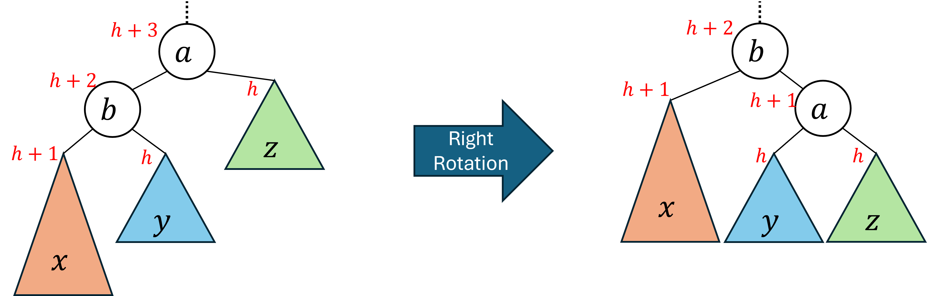
Notice that before the rotation, the node a was not balanced because its left subtree’s height was two more than its right subtree’s. We successfully rebalanced the tree by taking the tallest subtree (x, the left-left subtree of a) and moving it so it became a direct child of the root.
Also note that the rotation is guaranteed to preserve the binary search tree ordering property. From the original tree we know that the values must be in the order x < b < y < a < z. After the rotation we have x to the left of b, y to the left of a, a to the right of b, and z to the right of a, all of which are consistent with that ordering.
2.2.2 Left Rotation
A left rotation has the effect of lifting the right-right
subtree and dropping the left-left
subtree of the problem node.
The image below depicts a left rotation. Observe that before the rotation the problem node a is the root of the subtree. After the rotation its right child b becomes the root, and a becomes its left child. We call this a left rotation because the nodes shifted in a clockwise direction.
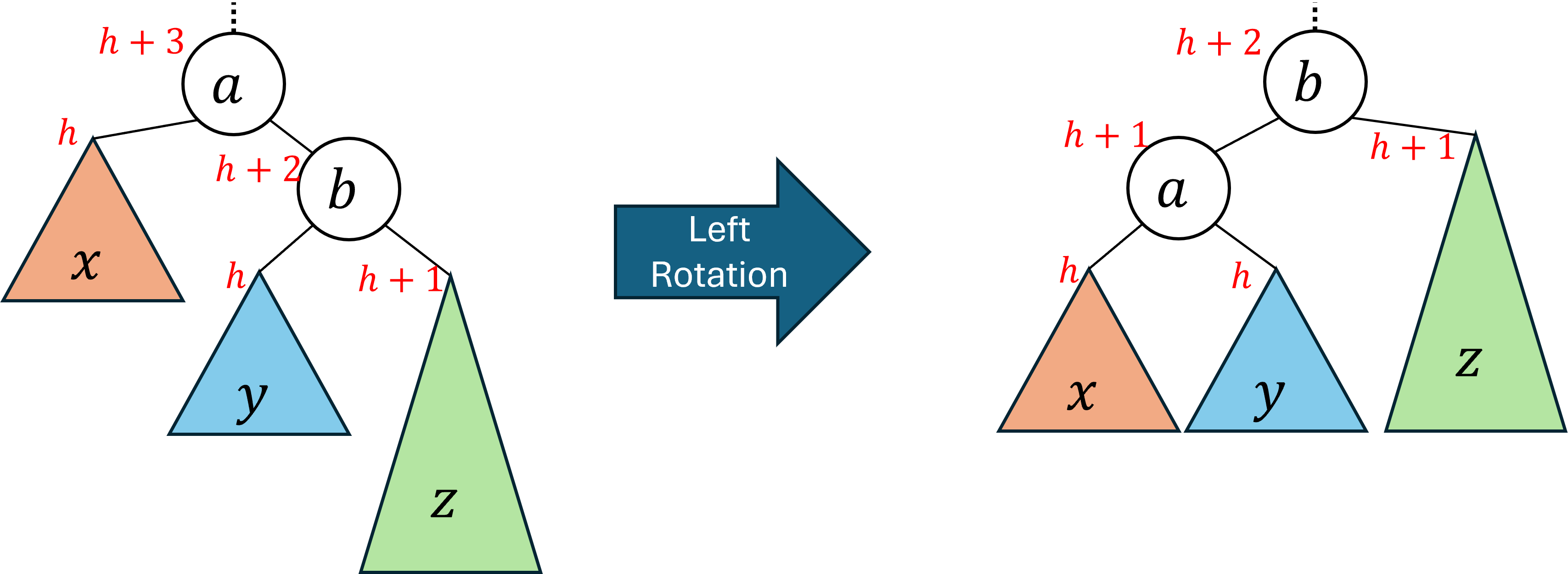
This rotation is exactly the mirror image of a right rotation, and so behaves following the exact same intuition.
2.2.3 Left-Right Rotation
We saw above that a left rotation raises the right-right subtree of the problem node and a right rotation raises the left-left subtree. Neither rotation impacts the level of the left-right or right-left subtrees of the problem node. To impact those subtrees we’ll need to use two rotations. We call this left-right rotation and the right-left rotation to follow double rotations, and intuitively they operate similarly to each other. Because we know that a left rotation overall raises the right side of the tree, and a right rotation raises the left side, we will use a combination of each to raise the middle
subtrees.
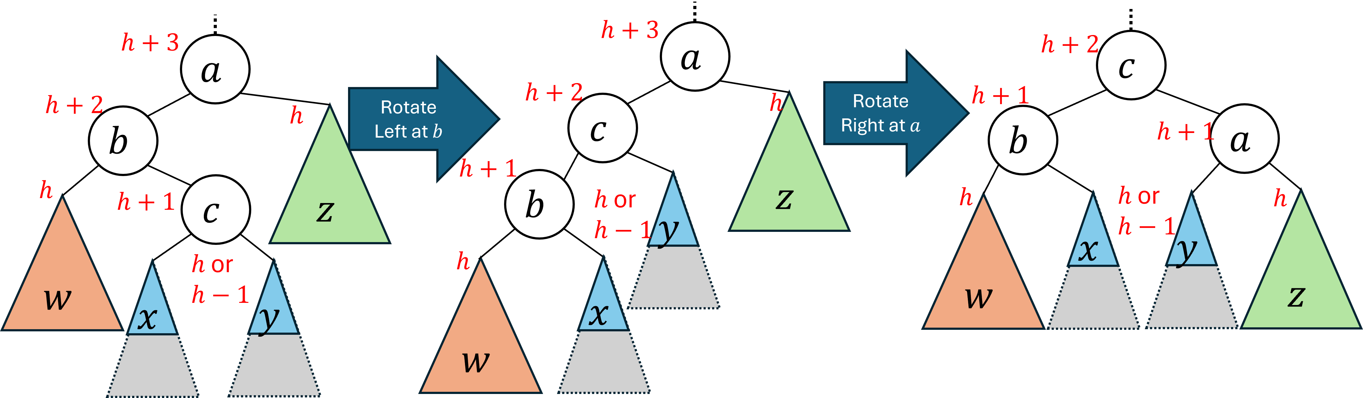
A left-right rotation has the effect of lifting the left-right subtree of the problem node (this is the subtree we get to by going from the problem node, to its left child, then to the child’s right subtree) in exchange for lowering the right subtree of the problem node. To do this we will first do a left rotation on the problem node’s left child. This has the impact of lifting the left-right subtree of the problem node, but comes at the expense of lowering the left-left subtree of the problem node. Because in this case it was the problem node’s left subtree that was too low, this may not have actually fixed the unbalance. To ensure the tree is balanced we will now do a right rotation at the problem node to lift that left-left subtree an lower the right-right subtree.
The image below depicts a left-right rotation. Observe that before the rotation the problem node a is the root of the subtree. After the rotation the node c, which is left-right grandchild of a, becomes the root of the subtree. The left-left subtree ends at exactly the same level as where it started. The right-right subtree is lower than it was previously. The original left-right subtree has been split
. The overall impact is that all nodes in the left-right subtree are higher than they were before the double rotation and the right subtree of the problem node is lower, therefore balancing the tree.
Because a left-right rotation is simply a left rotation followed by a right rotation, and we already established that both left and right rotations preserve the binary search tree ordering property, a left-right rotation will do so as well.
2.2.4 Right-Left Rotation
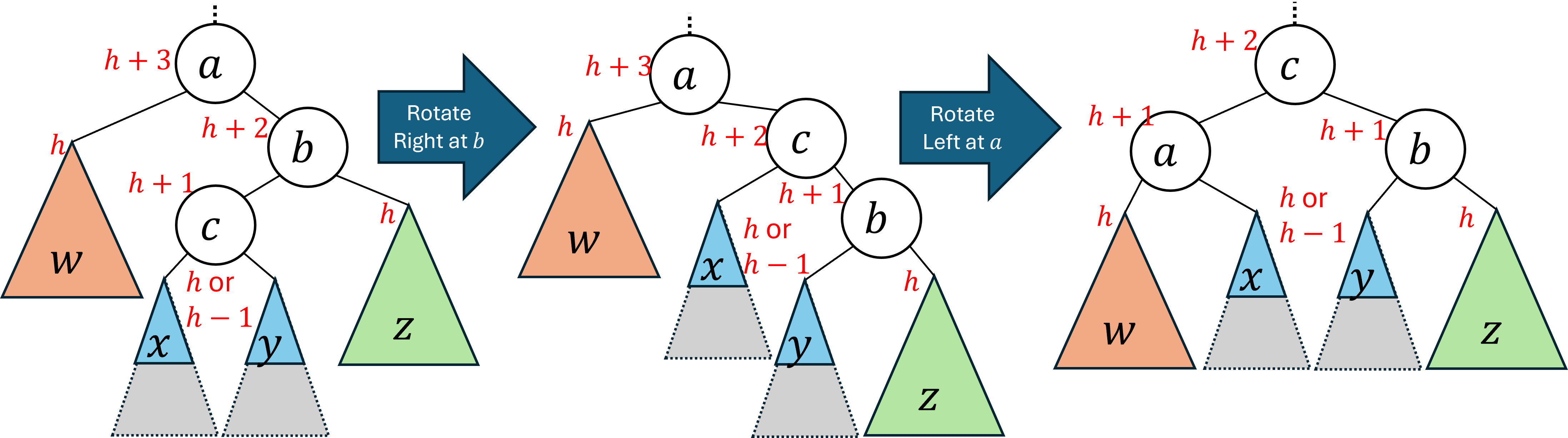
A right-left rotation is the mirror image of a left-right rotation. It has the overall effect of lifting the right-left subtree of the problem node in exchange for lowering the left subtree of the problem node. It operates by first doing a right rotation on the right child of a, and then doing a left rotation on a.
2.3 AVL Tree Insert
We now have all of the tools necessary in order to completely define our insert algorithm for AVL trees, which proceeds as follows:
- First perform a BST insert, which will either update the value associated with the given key, or else create a new node with the given key-value pair.
- If the key was already present in the tree, and we therefore updated the value associated with it, we did not modify the tree and therefore are finished with the insert.
- We we added a new node (which will always be a leaf) then we may have caused the AVL tree to become unbalanced, and so we must check for unbalance and perhaps perform rotations.
- Starting from the new leaf and moving one level at a time toward the root, check to see if any node is a
problem node
, meaning that the heights of its left and right subtrees differ by more than 1. - If the current node is a problem node, identify where the new node was added relative to that problem node:
- If the new node was added to the left-left subtree then do a right rotation.
- If the new node was added to the right-right subtree then do a left rotation.
- If the new node was added to the left-right subtree then do a left-right double rotation.
- If the new node was added to the right-left subtree then do a right-left double rotation.
To evaluate the running time of this algorithm we observe the following:
- A BST insert is linear in the height of the tree
- Supposing there is a height field within each node that is correctly maintained, step 4 requires only constant time per level
- Step 5 also requires constant time because each rotation requires only updating references and height fields for the nodes a, b, and c (in the case of a double rotation only).
Overall, the running time of an AVL tree insert is also linear in the height of the tree.
2.4 AVL Tree Delete
The AVL tree delete algorithm proceeds as follows:
- First perform a BST delete. If the key was not present then we do not modify the tree and therefore can return without any further steps. If the key was present then we removed a node from the tree, and so we may have caused the AVL tree to become unbalanced, and so we must check for unbalance and perhaps perform rotations.
- Starting from the parent of the node whose position was removed (if the key-value pair removed had either 0 or 1 child then we start from the parent of that node, if the key-value pair removed had two children then we start from the parent of where we found the largest node on the left) and moving one level at a time toward the root, check to see if any node is a
problem node
, meaning that the heights of its left and right subtrees differ by more than 1. - If the current node is a problem node, identify where the node was removed relative to that problem node:
- If the node was removed from the left-left subtree then do a left rotation.
- If the node was removed from the right-right subtree then do a right rotation.
- If the node was removed from the left-right subtree then do a right-left double rotation.
- If the node was removed from the right-left subtree then do a left-right double rotation.
Note that the cases for rotations are exactly the opposite of inserting relative to where the change happened (they are the same relative to which subtree was too tall/short).
Similar to inserting, we still do constant work per level of the tree, and so the running time is linear in the tree’s height.
2.5 Justifying Logarithmic Height
Now that we have established that, like with binary search trees, AVL tree operations run in linear time relative to the tree’s height, all that remains to justify our logarithm running time is an argument to show that the height of an AVL tree is logarithmic in terms of the number of nodes it contains.
Similar to what we did with heaps, we will begin by first fixing the height of the tree to h, and then identifying the minimum number of nodes that tree could contain. Because our running time is linear in the trees height, this will serve as a worst case analysis because that maximizes the height relative to the number of nodes.
We will define the function M(h) to return the minimum number of nodes in an AVL tree of height h. We can define M(h) using a recurrence relation as follows:
M(h) = M(h-1)+ M(h-2) + 1.
M(-1)=0, M(0)=1
Let’s discuss how we derived this. First of all, a tree of height -1 must have 0 nodes and a tree of height 0 must have exactly 1 node, giving the base cases of the recurrence.
For the recursive we’re saying that we can form the minimum-sized AVL tree of height h by first finding the minimum-sized AVL tree of height h-1 (which will have M(h-1) nodes) and of height h-2 (which will have M(h-2) nodes). Then we connect those together with a shared parent node (thus we add 1). This must be the minimum because for a tree to be height h at least one subtree of the root must have height h-1, and the other subtree must then have height h-1 or lower. Because an AVL tree requires that the height of sibling subtrees may differ by no more than 1, the minimum height of the other subtree is h-2.
From here, we can get an asymptotic lower bound on M(h) by comparing it to the Fibbonacci sequence.
The nth Fibbonacci number can be calculated following the recurrence:
F(n)=F(n-1)+F(n-2)
F(0)=0, F(1)=1
We can observe that for all values of x\geq 0 it holds that M(x)\geq F(x). This would be best justified using induction. We’ll skip a formal inductive proof and instead just provide a sketch of the argument. The inequality holds true for the base cases, and then for each application of the recursive case the M recurrence grows by 1 more than the Fibbonacci recurrence does.
We can then approximate the value of the nth Fibonacci number as F(n)\approx \phi^n where \phi=\frac{1=\sqrt{5}}{2}\approx 1.62 is the golden ratio.
Because M(x)\geq F(x), we can lower bound the minimum number of nodes in a tree of height h as \phi^h. Because the running time of our AVL tree operations are \Theta(h), we can define an upper bound on worst case the running time in terms of n by setting n=\phi^h, then solving for h. This gives a worst case running time of O(\log_\phi n)=O(\log n).
We can also get a \Omega bound on the worst case running time by observing that the maximum number of nodes in a tree of height h is 2^{h+1}-1. Setting n=2^{h+1}-1 and solving for h gives h=\log_2{n+1}-1, and so the worst case running time is \Omega(\log n). Because the running time is both O(\log n) and \Omega(\log n), we conclude the worst case running time is \Theta(\log n).