CSE 312 – Section 8 Solutions
Spring 2026
Review of Main Concepts
-
Multivariate: Discrete to Continuous:
Discrete Continuous Joint PMF/PDF \( p_{X,Y}(x,y) = \Pr (X = x,Y=y)\) \( f_{X,Y}(x,y) \neq \Pr (X = x,Y=y)\) Joint range/support \(\Omega _{X,Y}\) \(\{(x,y)\in \Omega _X\times \Omega _Y: p_{X,Y}(x,y)>0\}\) \(\{(x,y)\in \Omega _X\times \Omega _Y: f_{X,Y}(x,y)>0\}\) Joint CDF \(F_{X,Y}\left ( x,y \right ) = \sum _{t \leq x,s\le y}{p_{X,Y}(t,s)}\) \(F_{X,Y}\left ( x,y \right ) = \int _{- \infty }^{x}{\int _{-\infty }^y{f_{X,Y}\left ( t,s \right )dsdt}}\) Normalization \(\sum _{x,y}^{}{p_{X,Y}(x,y)} = 1\) \(\int _{- \infty }^{\infty }{\int _{-\infty }^\infty {f_{X,Y}\left ( x,y \right )dxdy}} = 1\) Marginal PMF/PDF \(p_X(x)=\sum _y{p_{X,Y}(x,y)}\) \(f_X(x)=\int _{-\infty }^\infty {f_{X,Y}(x,y)dy}\) Expectation \(\expect {g(X,Y)} = \sum _{x,y}{g(x,y)p_{X,Y}(x,y)}\) \(\expect {g(X,Y)}= \int _{- \infty }^{\infty }{\int _{-\infty }^{\infty }{g(x,y)f_{X,Y}( x,y)dxdy}}\) Independence \(\forall x,y, p_{X,Y}(x,y)=p_X(x)p_Y(y)\) \(\forall x,y, f_{X,Y}(x,y)=f_X(x)f_Y(y)\) must have \(\Omega _{X,Y}=\Omega _X\times \Omega _Y\) \(\Omega _{X,Y}=\Omega _X\times \Omega _Y\) - Law of Total Probability (r.v. version): If \(X\) is a discrete random variable, then \[\Pr (A)=\sum _{x\in \Omega _X}{\Pr (A|X=x)p_X(x)}\quad \quad \text {discrete $X$}\]
-
Continuous Law of Total Probability: \[\Pr (A)=\int _{x\in \Omega _X}{\Pr (A|X=x)f_X(x)dx}\]
There will be problems covering the following concepts (some of which have not yet been discussed in lecture) on the Section 9 worksheet:
- Conditional expectation: The expected value of random variable \(X\) given that event \(A\) has occurred, written \(\expect {X|A}\), is defined as \[\expect {X|A} = \sum _{x \in \Omega _X} x \cdot \Pr (X=x | A).\]
- Discrete Law of Total Expectation (event version): Let \(A_1 \ldots , A_n\) be a partition of the sample space. Then \[\expect {X}=\sum _{i=1}^n \expect {X|A_i} \Pr (A_i).\]
- Discrete Law of Total Expectation (r.v. version): Let \(X\) and \(Y\) be two random variables. Then \[\expect {X}=\sum _{y \in \Omega _Y} \expect {X|Y=y} \cdot \Pr (Y=y).\]
- Continuous Law of Total Expectation: \[\expect {X}=\int _{y \in \Omega _Y}{\expect {X|Y=y}f_Y(y)dy}\]
- Expected value of \(X\) conditioned on r.v. \(Y\): Suppose that \(Y\) is a random variable that takes values \(y_1, \ldots , y_k\). Then \(\expect {X|Y}\) is the following random variable \[\expect {X|Y} = \begin {cases} \expect {X|Y=y_1} & \text {with probability }\Pr (Y=y_1)\\ \expect {X|Y=y_2} & \text {with probability }\Pr (Y=y_2)\\ \ldots & \\ \expect {X|Y=y_k} & \text {with probability }\Pr (Y=y_k)\\ \end {cases}\]
- Law of total expectation (rewritten): Given the above definition, we can write \[\expect {X} = \expect {\expect {X | Y}} = \sum _{i=1}^k \expect {X|Y=y_i}\cdot \Pr (Y=y_i).\]
- Covariance: We may not get to this in class, but there is a problem on the pset about it. To find out more, check out section 5.4 in the Tsun book. And now the definition: For any two random variables \(X,Y\) the covariance is defined as \[\Covariance {X,Y}=\expect {(X-\expect {X})(Y-\expect {Y})}.\] It can also be shown that \[\Covariance {X,Y}=\expect {XY}- \expect {X}\expect {Y}.\]
-
Conditional distributions: We are not explicitly covering this topic in class, but it is highly recommended that you study it. Much of the above can be more appropriately rewritten in terms of conditional distributions. See Tsun, Section 5.3.
Discrete Continuous Conditional PMF/PDF \(p_{X|Y}(x|y)=\frac {p_{X,Y}(x,y)}{p_Y(y)}\) \(f_{X|Y}(x|y)=\frac {f_{X,Y}(x,y)}{f_Y(y)}\) Conditional Expectation \(\expect {X|Y=y}=\sum _{x}{xp_{X|Y}(x|y)}\) \(\expect {X|Y=y}=\int _{-\infty }^\infty {xf_{X|Y}(x|y)dx}\)
Plan for Section
- Content Review (Problem 1)
- Joint PMF’s (Problem 2) - do it fast
- Continuous joint density - Problem 6
- 3 points on a line - Problem 7
- Min and max of i.i.d. random variables - Problem 8 if time permits
We recommend that students look at the final problem for examples of how to set up the ranges of integration. Might be helpful on the homework.
1 Content Review
- a)
- Select one: Given two discrete random variables \(X\) and \(Y\), the joint CDF
is
- \(F_{X,Y}(x,y) = \sum _{t<x} p_{X,Y}(t,y)\)
- \(F_{X,Y}(x,y) = \sum _{s<y} p_{X,Y}(x,s)\)
- \(F_{X,Y}(x,y) = \sum _{t \le x}\sum _{s \le y} p_{X,Y}(t,s)\)
- \(F_{X,Y}(x,y) = p_{X,Y}(x,y)\)
The third answer follows directly from the definition of multivariate / joint distributions.
- b)
- Marginal PDF. Let \(X\) and \(Y\) be continuous random variables with joint PDF
\(f_{X,Y}(x,y)\). Which of the following correctly expresses the marginal PDF
\(f_X(x)\)?
- \(\int _{-\infty }^\infty f_{X,Y}(x,y) \,dx\)
- \(\int _{-\infty }^\infty f_{X,Y}(x,y) \,dy\)
- \(\frac {f_{X,Y}(x,y)}{f_Y(y)}\)
- \(\int _{-\infty }^x \int _{-\infty }^y f_{X,Y}(t,s) \,ds\,dt\)
Answer: \(\int _{-\infty }^\infty f_{X,Y}(x,y) \,dy\)
To find the marginal distribution of \(X\), you must "integrate out" the other variable, \(Y\), over its entire range. (Note: The first option incorrectly integrates out \(x\), which would leave a function of \(y\). The third option is the conditional PDF \(f_{X|Y}(x|y)\), and the fourth option is the joint CDF \(F_{X,Y}(x,y)\).) - c)
- Independence and Support. True or False: If the joint support \(\Omega _{X,Y}\) of
the random variables \((X,Y)\) is a circle defined by \(x^2 + y^2 \le 1\), and \(\Omega _X=\Omega _Y = [0,1]\) then \(X\) and \(Y\) are
independent.
- True
- False
Answer: False
For \(X\) and \(Y\) to be independent, their joint support must be the Cartesian product of their marginal supports (\(\Omega _{X,Y} = \Omega _X \times \Omega _Y\)). A circle is not the Cartesian product of \([0,1]\). - d)
- Continuous Law of Total Probability. Let \(A\) be an event and \(X\) be a
continuous random variable with PDF \(f_X(x)\). Which of the following is the
correct expression for the Continuous Law of Total Probability?
- \(\Pr (A) = \int _{-\infty }^\infty \Pr (A \mid X=x) \,dx\)
- \(\Pr (A) = \int _{-\infty }^\infty \Pr (A \cap X=x) f_X(x) \,dx\)
- \(\Pr (A) = \int _{-\infty }^\infty \Pr (X=x \mid A) \Pr (A) \,dx\)
- \(\Pr (A) = \int _{-\infty }^\infty \Pr (A \mid X=x) f_X(x) \,dx\)
Answer: \(\Pr (A) = \int _{-\infty }^\infty \Pr (A \mid X=x) f_X(x) \,dx\)
The Continuous Law of Total Probability scales the conditional probability of \(A\) given \(X=x\) by the density of \(X\) at \(x\), integrated over all possible values of \(X\). (Note: Option 1 is missing the density weighting. Option 2 incorrectly combines an intersection with the density function. Option 3 is a jumbled application of Bayes’ rule elements.)
2 Joint PMF’s
Suppose \(X\) and \(Y\) have the following joint PMF:
| X/Y | 1 | 2 | 3 |
| 0 | 0 | 0.2 | 0.1 |
| 1 | 0.3 | 0 | 0.4 |
- a)
- Identify the range of \(X\) (\(\Omega _X\)), the range of \(Y\) (\(\Omega _Y\)), and their joint range (\(\Omega _{X,Y}\)).
\(\Omega _X=\{0,1\}\), \(\Omega _Y=\{1,2,3\}\), and \(\Omega _{X,Y}=\{(0,2),(0,3),(1,1),(1,3)\}\)
- b)
- Find the marginal PMF for \(X\), \(p_X(x)\) for \(x\in \Omega _X\).
\[p_X(0)=\sum _y{p_{X,Y}(0,y)}=0+0.2+0.1=0.3\] \[p_X(1)=1-p_X(0)=0.7\]
- c)
- Find the marginal PMF for \(Y\), \(p_Y(y)\) for \(y\in \Omega _Y\).
\[p_Y(1)=\sum _x{p_{X,Y}(x,1)}=0+0.3=0.3\] \[p_Y(2)=\sum _x{p_{X,Y}(x,2)}=0.2+0=0.2\] \[p_Y(3)=\sum _x{p_{X,Y}(x,3)}=0.1+0.4=0.5\]
- d)
- Are \(X\) and \(Y\) independent? Why or why not?
No, since a necessary condition is that \(\Omega _{X,Y}=\Omega _X\times \Omega _Y\).
- e)
- Find \(\expect {X^3Y}\).
Note that \(X^3=X\) since \(X\) takes values in \(\{0,1\}\). \[\expect {X^3Y}=\expect {XY}=\sum _{(x,y)\in \Omega _{X,Y}}{xyp_{X,Y}(x,y)}=1\cdot 1\cdot 0.3+1\cdot 3\cdot 0.4=1.5\]
3 Trinomial Distribution
A generalization of the Binomial model is when there is a sequence of \(n\) independent trials, but with three outcomes, where \(\Pr (\text {outcome }i)=p_i\) for \(i=1,2,3\) and of course \(p_1+p_2+p_3=1\). Let \(X_i\) be the number of times outcome \(i\) occurred for \(i=1,2,3\), where \(X_1+X_2+X_3=n\). Find the joint PMF \(p_{X_1,X_2,X_3}(x_1,x_2,x_3)\) and specify its value for all \(x_1,x_2,x_3\in \mathbb {R}\).
We use a similar argument as for the binomial PMF. \(\binom {n}{ x_1,x_2,x_3}\) is the number of ways to select which of the \(n\) outcomes result in each of the 3 outcomes. Then, we multiply the probabilities of each trial being the corresponding outcome (e.g., \(p_1^{x_1}\) is the probability that all \(x_1\) trials end up being outcome 1). This gives use the following PMF: \[p_{X_1,X_2,X_3}(x_1,x_2,x_3)=\binom {n}{x_1,x_2,x_3}\prod _{i=1}^3{p_i^{x_i}}=\frac {n!}{x_1!x_2!x_3!}p_1^{x_1}p_2^{x_2}p_3^{x_3}\] where \(x_1+x_2+x_3=n\) and are nonnegative integers.
4 Do You “Urn” to Learn More About Probability?
Suppose that 3 balls are chosen without replacement from an urn consisting of 5 white and 8 red balls. Let \(X_i = 1\) if the \(i\)-th ball selected is white and let it be equal to 0 otherwise. Give the joint probability mass function of
- a)
- \(X_1, X_2\)
Here is one way of defining the joint pmf of \(X_1, X_2\) \[\Pr (X_1 = 1, X_2 = 1) = \Pr (X_1 = 1)\Pr (X_2 = 1 \mid X_1 = 1) = \frac {5}{13} \cdot \frac {4}{12} = \frac {20}{156}\] \[\Pr (X_1 = 1, X_2 = 0) = \Pr (X_1 = 1)\Pr (X_2 = 0 \mid X_1 = 1) = \frac {5}{13} \cdot \frac {8}{12} = \frac {40}{156}\] \[\Pr (X_1 = 0, X_2 = 1) = \Pr (X_1 = 0)\Pr (X_2 = 1 \mid X_1 = 0) = \frac {8}{13} \cdot \frac {5}{12} = \frac {40}{156}\] \[\Pr (X_1 = 0, X_2 = 0) = \Pr (X_1 = 0)\Pr (X_2 = 0 \mid X_1 = 0) = \frac {8}{13} \cdot \frac {7}{12} = \frac {56}{156}\]
- b)
- \(X_1, X_2, X_3\)
Instead of listing out all the individual probabilities, we could write a more compact formula for the pmf. In this problem, the denominator is always \(P(13,k)\), where \(k\) is the number of random variables in the joint pmf. And the numerator is \(P(5, i)\) times \(P(8,j)\) where \(i\) and \(j\) are the number of 1s and 0s, respectively. If we wish to compute \(p_{X_1, X_2, X_3}(x_1, x_2, x_3)\), then the number of 1s (i.e., white balls) is \(x_1 + x_2 + x_3\), and the number of 0s (i.e., red balls) is \((1-x_1) + (1-x_2) + (1-x_3)\). Then, we can write the pmf as follows: \[p_{X_1, X_2, X_3}(x_1, x_2, x_3) = \frac {10!}{13!} \cdot \frac {5!}{(5 - x_1 - x_2 -x_3)!} \cdot \frac {8!}{(5 + x_1 + x_2 + x_3)!}\]
5 Successes
Consider a sequence of independent Bernoulli trials, each of which is a success with probability \(p\). Let \(X_1\) be the number of failures preceding the first success, and let \(X_2\) be the number of failures between the first 2 successes. Find the joint pmf of \(X_1\) and \(X_2\). Write an expression for \(E[\sqrt {X_1 X_2}]\). You can leave your answer in the form of a sum.
\(X_1\) and \(X_2\) take on two particular values \(x_1\) and \(x_2\), when there are \(x_1\) failures followed by one success, and then \(x_2\) failures followed by one success. Since the Bernoulli trials are independent the joint pmf is \[p_{X_1, X_2}(x_1, x_2) = (1-p)^{x_1}p \cdot (1-p)^{x_2}p = (1-p)^{x_1 + x_2}p^2\] for \((x_1,x_2) \in \Omega _{X_1, X_2} =\{0,1,2,\ldots \}\times \{0,1,2,\ldots \}\) By the definition of expectation \[E[\sqrt {X_1X_2}] = \sum _{(x_1, x_2) \in \Omega _{X_1, X_2}} \sqrt {x_1x_2} \cdot (1-p)^{x_1 + x_2}p^2.\]
6 Continuous joint density
The joint density of \(X\) and \(Y\) is given by \[f_{X,Y} (x,y) = \begin {cases} xe^{-(x+y)} & x > 0,y > 0\\ 0 & \text {otherwise}. \end {cases}\] and the joint density of \(W\) and \(V\) is given by \[f_{W,V} (w,v) = \begin {cases} 2 & 0 < w < v, 0 < v < 1\\ 0 & \text {otherwise}. \end {cases}\] Are \(X\) and \(Y\) independent? Are \(W\) and \(V\) independent?
For two random variables \(X, Y\) to be independent, we must have \(f_{X,Y}(x, y) = f_X(x)f_Y(y)\) for all \(x \in \Omega _X,~y \in \Omega _Y\).
Let’s start with \(X\) and \(Y\) by finding their marginal PDFs. By definition, and
using the fact that the joint PDF is 0 outside of \(y > 0\), we get: \[f_X(x) = \int _0^{\infty } xe^{-(x+y)} dy = e^{-x}x\] We do the
same to get the PDF of \(Y\), again over the range \(x > 0\): \[f_Y(y) = \int _0^{\infty } xe^{-(x+y)} dx = e^{-y}\] Since \(e^{-x}x \cdot e^{-y} = xe^{-x - y} = xe^{-(x+y)}\) for all \(x,y>0\), \(X\) and \(Y\) are
independent.
We can see that \(W\) and \(V\) are not independent simply by observing that \(\Omega _W = (0,1)\) and \(\Omega _V = (0,1)\), but \(\Omega _{W,V}\) is not equal to their Cartesian product. Specifically, looking at their range of \(f_{W,V}(w,v)\). Graphing it with w as the "x-axis" and v as the "y-axis", we see that :
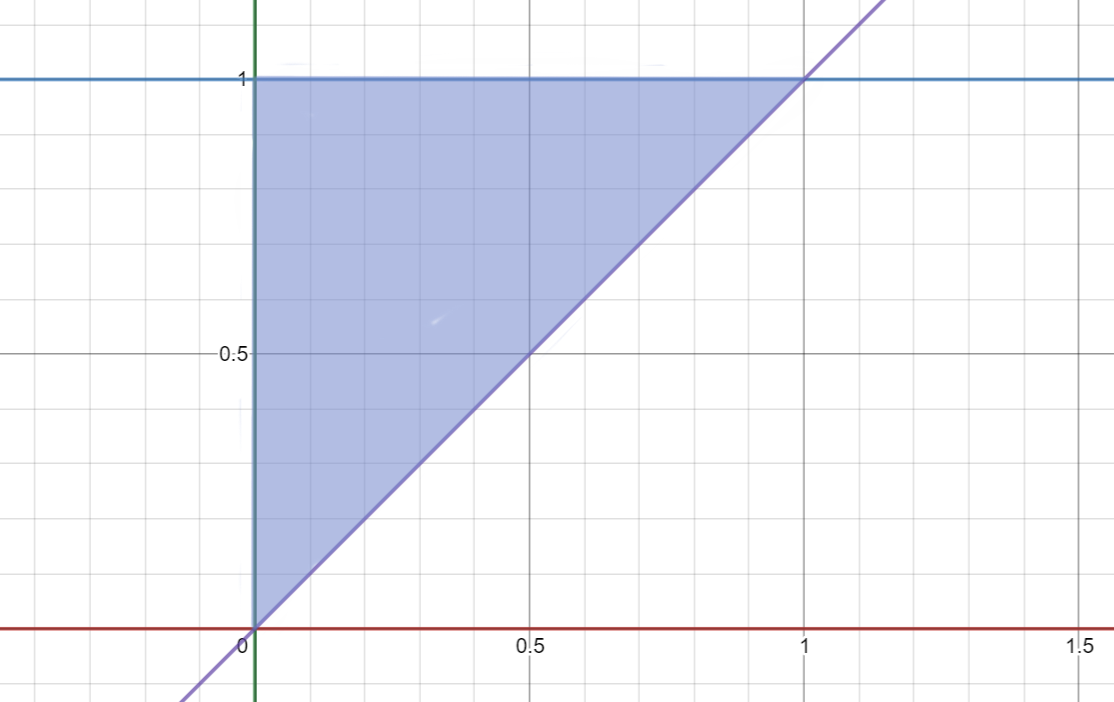
The shaded area is where the joint pdf is strictly positive. Looking at it, we
can see that it is not rectangular, and therefore it is not the case that \(\Omega _{W, V} = \Omega _W \times \Omega _V\).
Remember, the joint range being the Cartesian product of the marginal ranges is
not sufficient for independence, but it is necessary. Therefore, this is enough to
show that they are not independent.
7 3 points on a line
Three values \(X_1,X_2,X_3\) are selected uniformly at random, each between \(0\) and \(1\) (continuous independent uniform distributions). What is the probability that \(X_2\) is greater than \(X_1\) but less than \(X_3\)?
There are mutliple ways to approach this problem! Let \(X_1, X_2, X_3 \sim Unif(0, 1)\). We want to find \(\Pr (X_1 < X_2 < X_3)\).
Method 1: Condition on \(X_2\). \[ \begin {aligned} \Pr (X_1 < X_2 < X_3) &= \int ^\infty _{-\infty } \Pr (X_1 < X_2 < X_3 \mid X_2 = x) \; f_{X_2}(x) \; dx &\text {Continuous LoTP}\\ &= \int ^\infty _{-\infty } \Pr (X_1 < x, X_3 > x| X_2 =x) \; f_{X_2}(x) \; dx&\\ &= \int ^\infty _{-\infty } \Pr (X_1 < x, X_3 > x) \; f_{X_2}(x) \; dx&\text {Indep of $X_1,X_3$ from $X_2$}\\ &= \int ^\infty _{-\infty } \Pr (X_1 < x) \; \Pr (x < X_3) \; f_{X_2}(x) \; dx \quad &\text {Indep of $X_1,X_3$}\\ &= \int ^\infty _{-\infty } F_{X_1}(x) \; (1 - F_{X_3}(x))\; f_{X_2}(x) \; dx\\ &= \int ^1_{0} x \; (1 - x)\; 1 \; dx\\ &= \frac {x^2}{2} - \frac {x^3}{3} \bigg {|}^1_0 = \frac {1}{6} \end {aligned} \]
Method 2: Integrate over each variable. First, find the joint PDF of the three variables using independence \[f_{X_1,X_2,X_3}(x_1, x_2, x_3) = f_{X_1}(x_1)f_{X_2}(x_2)f_{X_3}(x_3) = \begin {cases} 1 & \text {if}\quad 0 \le x_1,x_2,x_3 \le 1 \\ 0 & \text {otherwise} \end {cases}\] So, the probability of the event \(X_1 < X_2 < X_3\) is exactly the volume of the region where \(x_1 < x_2 <x_2\). In order to integrate over these region, start with \(x_2\) (this has a range of \(0\) to \(1\)), then \(x_1\) (since \(x_1 < x_2\), its range is \(0\) to \(x_2\)), and finally \(x_3\) (since \(x_2 < x_3 < 1\), its range is \(x_2\) to \(1\)).
\[ \begin {aligned} \Pr (X_1 < X_2 < X_3) &= \int ^1_{0} \int ^{x_2}_{0} \int ^{1}_{x_2} f_{X_1, X_2,X_3}(X_1, X_2, X_3) \; dx_3dx_1dx_2 \\ &= \int ^1_{0} \int ^{x_2}_{0} \int ^{1}_{x_2} 1 \; dx_3dx_1dx_2 \\ &= \int ^1_{0} \int ^{x_2}_{0} x_3 \Bigg |_{x_2}^1dx_1 dx_2 = \int ^1_{0} \int ^{x_2}_{0} 1 - x_2 \; dx_1 dx_2\\ &= \int ^1_{0} (1-x_2)x_1 \Bigg |_{0}^{x_2} dx_2 = \int ^1_{0} (1 - x_2)x_2 \; dx_2\\ &= \frac {x^2}{2} - \frac {x^3}{2} \Bigg |_{0}^{1} = \frac {1}{6} \end {aligned} \]
Method 3: Identify symmetry. The key idea is to note that since \(X_1,X_2,X_3\) are i.i.d,
every ordered sequence is equally likely, i.e \(P(X_1 < X_2 < X_3) = P(X_1 < X_3 < X_2) = \dots =P(X_3 < X_2 < X_1)\).
Since there are \(3\) variables, there are \(3! = 6\) equally likely sequences. Also note that the \(6\) events are disjoint (no set of them can be occur simultaneously) and it is impossible for none of them to occur (ties like \(X_1=X_2\) have probability \(0\)). Therefore, they partition the sample space, so their probabilities should add up to \(1\). \[ \begin {aligned} 1 &= P(X_1 < X_2 < X_3)+ \dots +P(X_3 < X_2 < X_1) \quad &\text {Events partition the sample space} \\ &= 6 \cdot P(X_1 < X_2 < X_3) \quad &\text {Equally likely sequences} \\ &\implies P(X_1 < X_2 < X_3) = \frac {1}{6} \end {aligned} \]
8 Min and max of i.i.d. random variables
Let \(X_1, X_2, \ldots , X_n\) be i.i.d. random variables each with CDF \(F_X(x)\) and pdf \(f_X(x)\). Let \(Y= \min (X_1, \ldots , X_n)\) and let \(Z = \max (X_1, \ldots , X_n)\). Show how to write the CDF and pdf of \(Y\) and \(Z\) in terms of the functions \(F_X(\cdot )\) and \(f_X(\cdot )\).
First we compute the CDFs of \(Z\) and \(Y\) as follows: \[ \begin {aligned} F_Z(z) &= P(Z < z)\\ &= P(X_1 < z, ..., X_n < z) \quad &[\text {Definition of max}]\\ &= P(X_1 < z) \cdot ... \cdot P(X_n < z) \quad &[\text {Independence}]\\ &= (F_X(z))^n \end {aligned} \] \[ \begin {aligned} F_Y(y) &= P(Y < y)\\ &= 1 - P(Y > y)\\ &= 1 - P(X_1 > y, ..., X_n > y) \quad &[\text {Definition of min}]\\ &= 1 - P(X_1 > y) \cdot ... \cdot P(X_n > y) \quad &[\text {Independence}]\\ &=1 - (1 - F_X(y))^n \end {aligned} \] Using the fact that \(f_X(x) = \frac {d}{dx}F_X(x)\) and the CDFs that we found we can compute the pdfs of \(Z\) and \(Y\) as follows: \[ \begin {aligned} f_Z(z) &= \frac {d}{dz}F_Z(z)\\ &= \frac {d}{dz}(F_X(z))^n\\ &=n \cdot F_X(z)^{n-1} \cdot \left (\frac {d}{dz}F_X(z)\right )\\ &= n \cdot F_X(z)^{n-1} \cdot f_X(z) \end {aligned} \] \[ \begin {aligned} f_Y(y) &= \frac {d}{dy}F_Y(y)\\ &= \frac {d}{dy} \left (1 - (1 - F_X(y))^n\right )\\ &= -n \cdot (1 - F_X(y))^{n-1} \cdot \frac {d}{dy}(1 - F_X(y))\\ &= n \cdot (1 - F_X(y))^{n-1} \cdot f_X(y) \end {aligned} \]
9 Law of Total Probability
- a)
- Suppose we flip a coin with probability \(U\) of heads, where \(U\) is equally
likely to be one of \(\Omega _U=\{0,\frac {1}{n},\frac {2}{n},...,1\}\) (notice this set has size \(n+1\)). Let \(H\) be the event that
the coin comes up heads. What is \(\Pr (H)\)?
We can use the law of total probability, conditioning on \(U=\frac {k}{n}\) for \(k=0,...,n\). \[\Pr (H)=\sum _{k=0}^n{\Pr \left (H \mid U=\frac {k}{n}\right )\Pr \left (U=\frac {k}{n}\right )}=\sum _{k=0}^n{\frac {k}{n}\cdot \frac {1}{n+1}}\] \[=\frac {1}{n(n+1)}\sum _{k=0}^n{k}=\frac {1}{n(n+1)}\frac {n(n+1)}{2}=\frac {1}{2}\]
- b)
- Now suppose \(U\sim \textsf {Uniform(0,1)}\) has the continuous uniform distribution over the
interval \([0,1]\). Use the continuous law of total probability to handle this
case.
We can perform basically the same process as above, just using an integral instead of a sum. The values that \(U\) can take on are anywhere in the continuous interval \([0,1]\), so we integrate over that with respect to \(u\) and use the PDF of \(U\). Plugging that in we can get the same answer of \(\frac {1}{2}\) as before. \[\Pr (H)=\int _0^1{\Pr (H \mid U=u)f_U(u)du}=\int _0^1{u\cdot 1du}=\frac {1}{2}[u^2]^1_0=\frac {1}{2}\]
- c)
- Suppose that \(X_1\) and \(X_2\) are independent continuous random variables. Find an
expression for \(\Pr (X_{1} < {2X}_{2})\) using the law of total probability, in terms of \(F_{X_{1}},F_{X_{2}},f_{X_{1}},{f_{X}}_{2}\). (Your answer
will be in the form of a single integral, and requires no calculations – do not
evaluate it).
We use the continuous version of the “Law of Total Probability” to integrate over all possible values of \(X_2\): \[\Pr ( X_{1} < 2X_{2}) = \int _{- \infty }^{\infty }{\Pr ( X_{1} < 2X_{2} \mid X_{2} = x_{2})f_{X_{2}}( x_{2})dx_{2}} = \int _{- \infty }^{\infty }{F_{X_{1}}\left ( 2x_{2} \right )f_{X_{2}}\left ( x_{2} \right )dx_{2}}\]
- d)
- Suppose \(X_{1}\sim \mathcal {N}(\mu _{1},\sigma _{1}^{2})\) and \(X_{2}\sim \mathcal {N}(\mu _{2},\sigma _{2}^{2})\). Find \(s\), where \(\Phi \left ( s \right ) = \Pr (X_{1} < 2X_{2})\) using the fact that linear combinations of
independent normal random variables are still normal.
Let \(X_{3} = X_{1} - {2X}_{2}\), so that \(X_{3}\sim \mathcal {N}(\mu _{1} - 2\mu _{2},\sigma _{1}^{2} + 4\sigma _{2}^{2})\) (by the reproductive property of normal distributions)
\[\Pr ( X_{1} < 2X_{2}) = \Pr ( X_{1} - {2X}_{2} < 0) = \Pr ( X_{3} < 0) = \Pr \left ( \frac {X_{3} - \left ( \mu _{1} - 2\mu _{2} \right )}{\sqrt {\sigma _{1}^{2} + 4\sigma _{2}^{2}}} < \frac {0 - \left ( \mu _{1} - 2\mu _{2} \right )}{\sqrt {\sigma _{1}^{2} + 4\sigma _{2}^{2}}}\right )\]
\[= \Pr \left ( Z < \frac {2\mu _{2} - \mu _{1}}{\sqrt {\sigma _{1}^{2} + 4\sigma _{2}^{2}}}\right ) = \Phi \left ( \frac {2\mu _{2} - \mu _{1}}{\sqrt {\sigma _{1}^{2} + 4\sigma _{2}^{2}}} \right ) \implies s = \frac {2\mu _{2} - \mu _{1}}{\sqrt {\sigma _{1}^{2} + 4\sigma _{2}^{2}}}\]
- e)
- Suppose \(Z = X+Y\), where \(X\) and \(Y\) are independent. \(Z\) is called the convolution of the two
random variables. If \(X,Y,Z\) are discrete, using the law of total probability, we can
write \[p_{Z}\left ( z \right ) = \Pr ( X+Y = z) = \sum _{x}^{}{\Pr (X = x \cap Y = z - x)} = \sum _{x}^{}{p_{X}\left ( x \right )p_{Y}(z - x)}\] Write an analogous expression for \(F_Z(z)\) in the case that \(X,Y,Z\) are continuous
where, again, \(X\) and \(Y\) are independent.
\[F_{Z}\left ( z \right ) = \Pr ( X + Y \leq z ) = \int _{- \infty }^{\infty }{\Pr ( Y \leq z - X \mid X = x)f_{X}(x)dx} = \int _{- \infty }^{\infty }{F_{Y}(z - x)f_{X}(x)dx}\]
10 Jointly distributed random variables involving 3 variables
- a)
- Validating a Joint Density. Let \(X, Y\), and \(Z\) be continuous random
variables. To verify that \(f_{X,Y,Z}(x,y,z) = 6\) for the region \(0 \le x \le y \le z \le 1\) (and \(0\) otherwise) is a valid joint
probability density function, which of the following equations must hold
true?
- \(\int _{0}^{1} \int _{0}^{1} \int _{0}^{1} 6 \,dx \,dy \,dz = 1\)
- \(\int _{0}^{1} \int _{0}^{z} \int _{0}^{y} 6 \,dx \,dy \,dz = 1\)
- \(\int _{0}^{1} \int _{0}^{x} \int _{0}^{y} 6 \,dz \,dy \,dx = 1\)
- \(\int _{0}^{1} \int _{x}^{1} \int _{y}^{1} 6 \,dx \,dy \,dz = 1\)
Answer: \(\int _{0}^{1} \int _{0}^{z} \int _{0}^{y} 6 \,dx \,dy \,dz = 1\)
To be a valid joint PDF, the integral of the density over the entire valid region must equal \(1\). The support is given by the chain of inequalities \(0 \le x \le y \le z \le 1\). Setting up the bounds from the outside in using the order \(dx \,dy \,dz\): the outermost variable \(z\) ranges from absolute minimum to maximum (\(0\) to \(1\)). For a fixed \(z\), the variable \(y\) is bounded between \(0\) and \(z\). Finally, for fixed \(y\) and \(z\), the innermost variable \(x\) is bounded between \(0\) and \(y\). \[ \int _{0}^{1} \int _{0}^{z} \int _{0}^{y} 6 \,dx \,dy \,dz = 1 \] - b)
- Integrating out a Variable. Let \(X, Y\), and \(Z\) be continuous random
variables with joint PDF \(f_{X,Y,Z}(x,y,z) = 6\) for the region \(0 \le x \le y \le z \le 1\), and \(0\) otherwise. Which of the
following correctly expresses the joint marginal PDF \(f_{X,Y}(x,y)\) for the valid
region?
- \(\int _{0}^{1} 6 \,dz\)
- \(\int _{x}^{y} 6 \,dz\)
- \(\int _{0}^{y} 6 \,dz\)
- \(\int _{y}^{1} 6 \,dz\)
Answer: \(\int _{y}^{1} 6 \,dz\)
To find the joint marginal PDF \(f_{X,Y}(x,y)\), we must "integrate out" the variable \(Z\) over its valid range. Given the support bounds \(0 \le x \le y \le z \le 1\), for any fixed values of \(x\) and \(y\), the variable \(z\) ranges from a minimum of \(y\) to a maximum of \(1\). \[ f_{X,Y}(x,y) = \int _{y}^{1} f_{X,Y,Z}(x,y,z) \,dz = \int _{y}^{1} 6 \,dz \] (Note: The bounds are the key trap here. Because the joint PDF is only non-zero when \(z \ge y\), the lower limit of integration must be \(y\), not \(0\) or \(x\).) - c)
- The 3D Simplex. Let \(X, Y\), and \(Z\) be independent random variables, each
uniformly distributed over \((0,1)\). Which of the following integrals correctly
computes the probability that \(X + Y + Z \le 1\)?
- \(\int _{0}^{1} \int _{0}^{1} \int _{0}^{1} 1 \,dz \,dy \,dx\)
- \(\int _{0}^{1} \int _{0}^{1-x} \int _{0}^{1-x-y} 1 \,dz \,dy \,dx\)
- \(\int _{0}^{1} \int _{0}^{x} \int _{0}^{y} 1 \,dz \,dy \,dx\)
- \(\int _{0}^{1} \int _{0}^{1-x} \int _{0}^{1} 1 \,dz \,dy \,dx\)
Answer: \(\int _{0}^{1} \int _{0}^{1-x} \int _{0}^{1-x-y} 1 \,dz \,dy \,dx\)
First, the joint density of \(X,Y,Z\) is \(f_{X,Y,Z}(x,y,z) = 1\) due to independence and standard uniform distributions. We need to integrate this density over the region where \(X + Y + Z \le 1\). If we fix the outer bounds for \(X=x\) from \(0\) to \(1\), the remaining "budget" for \(Y\) is \(1-x\), so \(Y\) integrates from \(0\) to \(1-x\). Finally, given \(X=x\) and \(Y=y\), the variable \(Z\) is bounded above by \(1-x-y\). \[ \Pr (X + Y + Z \le 1) = \int _{0}^{1}\int _{0}^{1-x}\int _{0}^{1-x-y} 1 \,dz \,dy \,dx \] - d)
- Bounding with Max. Let \(X, Y\), and \(Z\) be independent random variables, each
uniformly distributed over \((0,1)\). Which of the following integrals correctly
computes \(\Pr (X \ge \max (Y, Z))\)?
- \(\int _{0}^{1} \int _{x}^{1} \int _{x}^{1} 1 \,dz \,dy \,dx\)
- \(\int _{0}^{1} \int _{0}^{1} \int _{0}^{\max (y,z)} 1 \,dx \,dy \,dz\)
- \(\int _{0}^{1} \int _{0}^{x} \int _{0}^{x} 1 \,dz \,dy \,dx\)
- \(\int _{0}^{1} \int _{0}^{1} \int _{\min (y,z)}^{1} 1 \,dx \,dy \,dz\)
Answer: \(\int _{0}^{1} \int _{0}^{x} \int _{0}^{x} 1 \,dz \,dy \,dx\)
The joint density is \(f_{X,Y,Z}(x,y,z) = 1\). The condition \(X \ge \max (Y, Z)\) is equivalent to stating that \(X \ge Y\) and \(X \ge Z\). It is easiest to set \(x\) as the outermost integral bounding from \(0\) to \(1\). Then, for any fixed value of \(X=x\), both \(Y\) and \(Z\) are independently bounded to be less than or equal to \(x\). Thus, \(y\) ranges from \(0\) to \(x\), and \(z\) ranges from \(0\) to \(x\). \[ \Pr (X \ge \max (Y, Z)) = \int _{0}^{1}\int _{0}^{x}\int _{0}^{x} 1 \,dz \,dy \,dx \] - e)
- Conditional PDF. (Not covered in class.) For two continuous random
variables \(X\) and \(Y\), which of the following defines the conditional PDF
\(f_{X|Y}(x|y)\)?
- \(\frac {f_{X,Y}(x,y)}{f_X(x)}\)
- \(\frac {f_{X,Y}(x,y)}{f_Y(y)}\)
- \(f_X(x)f_Y(y)\)
- \(\int _{-\infty }^\infty f_{X,Y}(x,y) \,dy\)
Answer: \(\frac {f_{X,Y}(x,y)}{f_Y(y)}\)
The conditional PDF of \(X\) given \(Y=y\) is the joint PDF divided by the marginal PDF of \(Y\) evaluated at \(y\). (Note: Option 1 is \(f_{Y|X}(y|x)\), option 3 is the joint PDF only if \(X\) and \(Y\) are independent, and option 4 is the marginal PDF of \(X\).)