The content for this lesson is adapted from material by Hunter Schafer and by Kevin Lin.
Objectives
By the end of this lesson, students will be able to:
- Describe the shape of a vector representing an unrolled grayscale or color image.
- Identify neural network model parameters and hyperparameters.
- Trace the execution of a small neural network given an input data point.
Setting up
To follow along with the code examples in this lesson, please download the files in the zip folder here:
Make sure to unzip the files after downloading! The following are the main files we will work with:
lesson21.ipynb
ML Review
Machine learning (ML) uses features of a dataset and a learning algorithm to learn a target concept to predict the label for a given example.
A model (the result of running a learning algorithm), is a concrete set of rules to take an example (maybe from the dataset) and predict the label. We might train a DecisionTreeClassifier on a dataset about surviving the sinking of the Titanic to create a specific model that can predict survival for data of that type.
The term model is often overloaded when discussed by machine learning practitioners. They sometimes refer to the specific model learned after training (e.g. this specific DecisionTreeClassifier that is the result of training on this data). Other times, they refer to the type of models you are considering (e.g. we are looking over the space of all DecisionTreeClassifiers of height at most 5 to find which one is best for this specific task). It is often confusing to figure out if they are talking about a specific model or a class of models. We commonly use the terminology of “model” to refer to a specific model and “model class” to refer to the class of all models of some type.
A dataset has features and labels. We always split a dataset into a training set and a test set. The training set is used by the learning algorithm to train the model. The test set is used to assess the model’s performance on data it did not train on, in order to get an unbiased estimate of its future performance.
The parameters of a model are the details of how a particular model is specified. For example, the parameters of a decision tree model are all of the split points and stop points in the tree. An alternative way of phrasing the learning algorithm is an algorithm that tries to find the optimal setting of the parameters (e.g. what the split and stop points should be) to maximize the accuracy. The hyperparameters of a model are the parameters you specify as a programmer to control which models can be selected. For example, setting the maximum height of the decision tree is a hyperparameter you choose that then effect which parameterization is chosen by the learning algorithm. Parameters are learned by the learning algorithm while hyperparameters are specified by the programmer.
So far, we’ve only used CSV datasets for machine learning, where we were able to use categorical, ordinal, and quantitative values to determine properties of our data that would lead to meaningful splits in a decision tree.
Vectorization
When working with images, it’s a little less clear on how to define machine learning features. Suppose we wanted to train a classifier to tell dog images from cat images. We would somehow need to derive features from the image that would be useful in predicting if the image contains a dog or a cat. It is fairly difficult to define features that are unique to dogs and also understandable by a decision tree. It’s hardly clear at all how we could begin to write code to take pixels from an image to produce those features! Instead, let’s have the machine learning algorithm try to learn how to predict the label from the image itself. To do this, we’ll need to to learn two new ML topics.
- Vectorization is the process of “flattening” or “unrolling” a multi-dimensional image data so that it can be more easily fed to a machine learning algorithm.
- Neural networks are a very powerful model class that can be used to learn high-level concepts from low-level features like pixels.
The idea behind vectorization is to “unroll” the image so instead of having 2-dimensions, it only has 1. Pictorially for a very small example image, this looks like the image below. We call this unrolled image a vector.
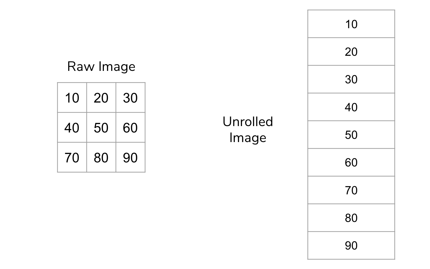
Most machine learning models are generic enough to take any series of features and learn a model from them. By unrolling the image, we have created a feature for every pixel in the image. Color images unroll the same way: each color channel is flattened into the same vector.
Since images can easily have hundreds of thousands or millions of pixels, our vectors will be just as large; this would overwhelm our linear regression algorithms! We’ll need more complex machine learning algorithms with many more parameters to deal with this overwhelming number of features.
Neural Networks
To introduce yourself to Neural Networks, we want you to watch a video from a YouTube channel called 3Blue1Brown. To help you focus your study, read these lists of questions and key ideas before watching the video. They probably won’t make much sense yet, so after watching the video, review these key points.
Note
In the video, grayscale images are represented as decimal values between 0.0 (black) and 1.0 (white) rather than 0 to 255.
Pay attention to…
- The general structure of a neural network and how it is used to make predictions.
- How many input neurons will there be for the digit recognition? Why that number?
- Why are there 10 output neurons for the digit recognition task?
- What is a hidden layer?
- How does the information go from one layer to the next?
- What is the intuition for why organizing the nodes in layers helps?
- How does a node determine its output value from its inputs?
Skim…
- The specific formula for the “squishing function” called the Sigmoid. All you really need to know is the general idea that it squishes the input to output between 0 and 1.
- 13:30 - 15:00 talks a bit about representing this process using matrices and vectors which is more complex than we care about. You should still watch the part after that since it shows a quick application of numpy and gives some more high-level motivation!
There is a whole series of videos that you are welcome to watch if you’re interested, but we will only focus on the first one.
Neural Networks Code
Let’s explore an example of a model that classifies handwritten digits (0-9) using the MNIST dataset. We’ll start by importing some libraries.
import math

import imageio.v3 as iio
import matplotlib.pyplot as plt
import numpy as np

from sklearn.datasets import fetch_openml # new! this is where the MNIST dataset comes from
from sklearn.model_selection import train_test_split

%matplotlib inline
Then, we load in the MNIST dataset, which contains hand-written digits with the labels of what each digit is. Each example is a 28x28 greyscale image, and its label is a number from 0 to 9. As mentioned above, it’s common to start by “unrolling” images for machine learning. The return value for the training set will be an ndarray with the shape (n, 784) where n is the number of examples in the dataset.
Food for thought: Why 784?
x, y = fetch_openml('mnist_784', version=1, return_X_y=True)
x = x / 255.  # scaling range of inputs to be between 0 and 1
Now, rather than using train_test_split as we normally would, we’ll use the first 60,000 rows of the MNIST dataset as our training data and the remainder as the test data. This is not a good idea in practice, but this particular dataset is provided by the author with those rows specifically to be used as the test set!
x_train = x[:60000]
x_test = x[60000:]
y_train = y[:60000]
y_test = y[60000:]

print(x_train.shape)
Note that checking the .shape attribute confirms the shape of the array that we described earlier! We can also use reshape to plot what the image looks like. Matplotlib’s imshow function will display images, and we’ll use the cmap parameter to enforce a greyscale rendering:
plt.imshow(np.array(x.iloc[2]).reshape((28, 28)), cmap=plt.cm.gray)
Pretty neat! Let’s create a neural network using sklearn. The specific model class that we’ll use is called a multi-layer perceptron, which is abbreviated to MLP.
Now, the most important parameter in this function is hidden_layer_sizes, which specifies the number of hidden layers and the number of nodes that appear at each layer. The remaining parameters are no less important, but we have chosen them specifically to keep the output manageable.
max_itergives the number of iterations, or the number of times the model updates its own parameters.verbosetells whether to print progress messages, like telling the user which iteration the model is onrandom_statedetermines random number generation for initializing the weights and bias in the model, so that the model has somewhere to start.
Note that these extra parameters are technically hyperparameters, since they are values we are setting to specify the type of model we want. Here, by passing in hidden_layer_sizes=(50,), we are creating a neural network with one hidden layer, and that hidden layer has 50 nodes. The number of input and output neurons is determined by sklearn using the provided data. Here, our network will have 784 input neurons (one per pixel), a layer of 50 neurons, and then 10 output neurons (one for each digit). You can think of output neurons like being the labels!
from sklearn.neural_network import MLPClassifier

mlp = MLPClassifier(hidden_layer_sizes=(50,),
                    max_iter=10, verbose=10, random_state=1)

mlp
We can then train our model on the training set and then check its train vs. test accuracy are. Here are some things to be mindful of:
- When running
fit, the model prints out lines beginning with “Iteration:…” This signifies each phase of updating the network weights based on misclassified examples. The loss is a measurement of how much error there is (but slightly different than accuracy) - With this particular arcitecture, we get really high accuracy for both the training and testing sets!
mlp.fit(x_train, y_train)
print(f"Training score: {mlp.score(x_train, y_train)}")
print(f"Testing score: {mlp.score(x_test, y_test)}")
These networks are quite sensitive to hyperparameters. If we add more layers and shorten the number of nodes in each layer, we can get a pretty different accuracy! Let’s try modifying the network architecture to have 5 hidden layers of 10 nodes each instead (still 50 hidden nodes, but in a different setup).
mlp2 = MLPClassifier(hidden_layer_sizes=(10, 10, 10, 10, 10),
                     max_iter=10, verbose=True, random_state=1)
mlp2.fit(x_train, y_train)


print(f"Training score: {mlp2.score(x_train, y_train)}")
print(f"Testing score: {mlp2.score(x_test, y_test)}")
This is why neural networks can be so complex! It’s hard to predict how changing the network architecture will affect the performance of the model. TensorFlow has a playground that uses a lot of knobs to tune for a neural network, and it’s touch to predict how the output will be affected by your choice of settings!
Food for thought: Try out a few different settings for the TensorFlow playground. What do you notice?

Hyperparameter Tuning
Since there’s really no one way of telling “what the best settings are”, one method that we can try is just to implement them all and see which one is best. For this example, we’ll try a few different network architectures, as well as modifying a new parameter called learning_rate, which essentially controls how much we update the weights on each iteration.
The nested loop below tries every possible setting; it’s a fairly common piece of ML code where we have to try all combinations of hyperparameters.
# learning_rate and size were somewhat arbitrarily chosen here
learning_rates = [0.001, 0.01, 0.5]
sizes = [(10,), (50,), (10, 10, 10, 10)]

for learning_rate in learning_rates:
    for size in sizes:
        print(f"Learning Rate: {learning_rate}, Size: {size}")
        mlp = MLPClassifier(hidden_layer_size=size, learning_rate_init=learning_rate,
                            max_iter=10, random_state=1)
        mlp.fit(x_train, y_train)
        print(f"    Training set score: {mlp.score(x_train, y_train)}")
        print(f"    Test set score: {mlp.score(x_test, y_test)}")
But wait! If we use the testing set in each combination of hyperparameters, then it’s no longer useful to us as a testing set! Remember, the purpose of having a testing set at all was to give an estimate of how our model will do in the future. If we choose hyperparameters based on that testing accuracy, then it’s no longer a good estimate of how the model will perform on future data.
In practice, we might actually set aside another portion of the training set as a validation set that we use to pick the hyperparameter settings. Then, we can leave the test set untouched until the very end of the project! At that point, we can test our final model and get a more accurate estimate of its performance in the future!
⏸️ Pause and 🧠 Think
Take a moment to review the following concepts and reflect on your own understanding. A good temperature check for your understanding is asking yourself whether you might be able to explain these concepts to a friend outside of this class.
Here’s what we covered in this lesson:
- Vectorization
- Neural network concepts
- MLP Classifier using MNIST data
- Hyperparameter tuning
- Validation set
Here are some other guiding exercises and questions to help you reflect on what you’ve seen so far:
- In your own words, write a few sentences summarizing what you learned in this lesson.
- What did you find challenging in this lesson? Come up with some questions you might ask your peers or the course staff to help you better understand that concept.
- What was familiar about what you saw in this lesson? How might you relate it to things you have learned before?
- Throughout the lesson, there were a few Food for thought questions. Try exploring one or more of them and see what you find.
In-Class
When you come to class, we will work together on completing the conceptual questions in today’s Canvas Quiz!
Canvas Quiz
All done with the lesson? Complete the Canvas Quiz linked here!