Lesson 20. Convolutions

The content for this lesson is adapted from material by Hunter Schafer.

Objectives¶

By the end of this lesson, students will be able to:

• Apply numpy and ndarray calculation functions.
• Trace the execution of a convolution on an image with a kernel.
• Apply a convolution operation on an image with a kernel.

Setting up¶

To follow along with the code examples in this lesson, please download the files in the zip folder here:

• lesson20.zip

Make sure to unzip the files after downloading! The following are the main files we will work with:

• lesson20.ipynb
• convolutions.ipynb

NumPy Functions¶

In lesson 19, we learned how images can be represented as numpy ndarray objects.

• 2-dimensional ndarrays for grayscale images. The shape of the image will be (height, width).
• 3-dimensional ndarrays for color images. The shape of the image will be (height, width, 3) where the innermost dimension has shape 3 for each color channel RGB.

There is a lot of syntax, but it’s quite similar to what we have seen previously with pandas, since pandas was built on top of numpy. You can think of this as pandas inheriting or extending numpy functionality and classes, which is why many function names, syntax, and data structures look similar.

In fact, many of the functions that we learned for aggregating values in pandas have their foundations in numpy. We can still use functions like max, min, mean, and sum directly on ndarrays:

import numpy as np
x = np.arange(10)

print(x.sum())
print(x.max())
print(x.min())
print(x.mean())

# use .prod for products
print(x.prod())

# and .std for standard deviation
print(x.std())

Or we can call these functions from the numpy library itself and pass in an ndarray as the parameter to that function. Either syntax achieves the same behavior!

print(np.sum(x))
print(np.max(x))
print(np.min(x))
print(np.mean(x))
print(np.prod(x))
print(np.std(x))

Food for thought: Which syntax do you prefer? Why do you think there are two syntaxes for the same functionality?

axis¶

Many of these functions accept an optional axis parameter that controls which dimension is collapsed. This is especially useful for images, where we might want to aggregate rows separately from columns.

image = np.array([
    [10, 20, 30],
    [40, 50, 60],
    [70, 80, 90]
])

# One sum per column with axis=0
print(np.sum(image, axis=0))  # [120, 150, 180]

# One sum per row with axis=1
print(np.sum(image, axis=1))  # [60, 150, 240]

# No axis argument collapses everything into a single value
print(np.sum(image))  # 450

A helpful way to think of it is that axis=0 moves down the rows, and axis=1 moves across the columns.

Convolutions¶

Our study of images so far has focused on pixel-by-pixel processing. However, as we saw with machine learning processing things one pixel at a time makes it hard to answer questions about our image data. There are just too many pixels in an image (a 1000-by-1000 image has 1 million pixels!) for programmers to work with manually.

Instead, we’ll need to build abstractions to identify local information in an image. An example of local information would be a question of the form, “Is there an edge in this part of the image?” This type of question is the foundation for machine learning image recognition systems known as convolutional neural networks. The type of operation we are going to describe here is the fundamental operation in this machine learning system called a convolution.

A convolution is a special way of looping over the pixels in an image. Instead of looping over an image one pixel at a time, a convolution loops over an image one subimage (sliced portion of the image) at a time. We call a convolution a sliding window algorithm because the algorithm starts at the top row, generates the first subimage for the top leftmost corner, then slides over 1 pixel to the right, and repeats the process.

# Print all 3x3 subimages in the 5x5 image
subimage_height = subimage_width = 3
image = np.array([
    [3, 3, 2, 1, 0],
    [0, 0, 1, 3, 1],
    [3, 1, 2, 2, 3],
    [2, 0, 0, 2, 2],
    [2, 0, 0, 0, 1]
])
image_height, image_width = image.shape
for i in range(image_height - subimage_height + 1):
    for j in range(image_width - subimage_width + 1):
        subimage = image[i:i + subimage_height, j:j + subimage_width]
        print((i, j))
        print(subimage)
        print()

So we now have a way to operate on subimages rather than individual pixels. But how do we apply an operation to each subimage? In a convolution, we use another 2-d array called a kernel that operates on each subimage. The result of a convolution is a smaller data array that stores the result of applying the kernel to each subimage.

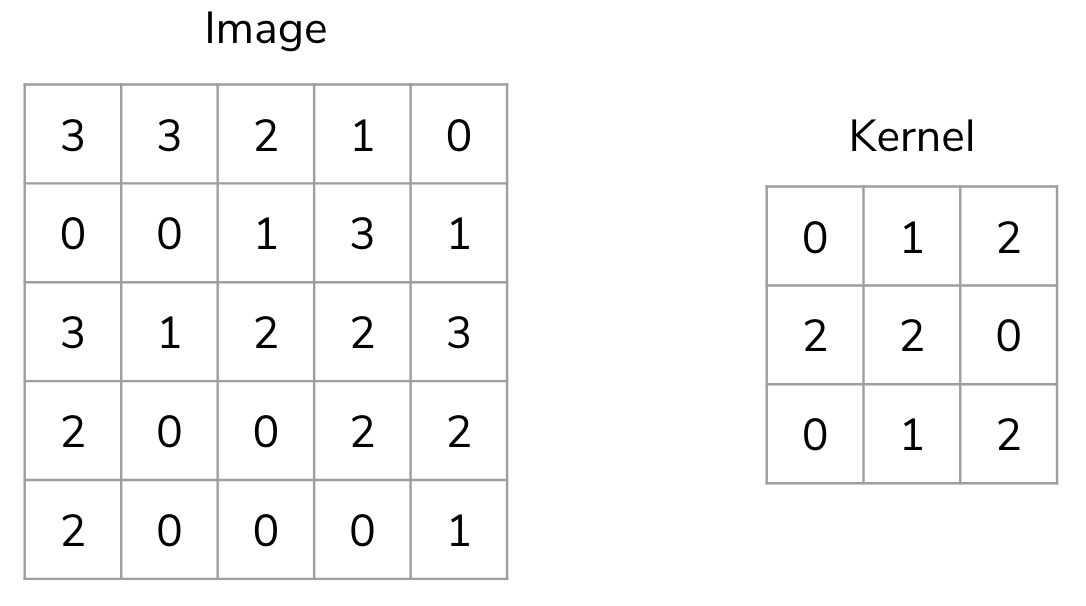
The kernel is applied to each subimage as the sum of element-wise products between subimage * kernel.

kernel = np.array([
    [0, 1, 2],
    [2, 2, 0],
    [0, 1, 2]
])
kernel_height, kernel_width = kernel.shape

image = np.array([
    [3, 3, 2, 1, 0],
    [0, 0, 1, 3, 1],
    [3, 1, 2, 2, 3],
    [2, 0, 0, 2, 2],
    [2, 0, 0, 0, 1]
])
image_height, image_width = image.shape

result_height = image_height - kernel_height + 1
result_width = image_width - kernel_width + 1
result = np.zeros((result_height, result_width))
for i in range(result_height):
    for j in range(result_width):
        subimage = image[i:i + kernel_height, j:j + kernel_width]
        result[i, j] = np.sum(subimage * kernel)
print(result)

For the [0, 0] index in the result ndarray, we can consider the calculation as follows:

$(3 \cdot 0) + (3 \cdot 1) + (2 \cdot 2) +\\ (0 \cdot 2) + (0 \cdot 2) + (1 \cdot 0) + \\ (3 \cdot 0) + (1 \cdot 1) + (2 \cdot 2) = 12$

Because a convolution computes a value for each subimage, the result depends on the choice of kernel. Each value in the result can reveal something meaningful about the original image!

Kernel Examples¶

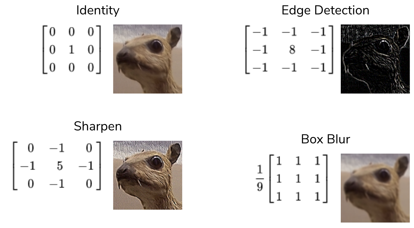
There are many kernels that are used in practice, with many different sizes, but we will discuss four examples of 3x3 kernels.

1. Identity. This is a kernel with a 1 in the center, surrounded by 0s. This results in the same image, though perhaps with some pixels cropped-out at the edges. The result of the convolution will only be the value of the center pixel; the others are “dropped”.
2. Edge detection. This is a kernel with 8 in the center, surrounded by -1. If all values are the same (i.e., all 9 values in the subimage are the same color), then the 8 -1 values cancel out the +8 value in the center. If there is a difference in the color values, then some difference shows up in the result at that window location.
3. Sharpen. Similar to the edge detection kernel, there is a 5 in the center, surrounded by alternating 0 and -1. The center pixel is “weighted” more, while the surrounding pixels are weighted less or dropped.
4. Box blur. A kernel of 1s, multiplied by 1/9. Essentially, this kernel takes the average of all 9 pixels in that window location and blurs the image by taking the “average” color in that location.

Why Convolutions?¶

How do we write a program to determine if a given image contains a dog or a cat? If you asked a computer vision scientist a couple decades ago, they might have answered by designing features using convolutions with different kernels to detect corners or edges and then define an algorithm to combine the different result arrays together. Just like how visual cognition works by combining many simple line detectors, kernels work by specifying specific edge detectors define meaningful features. However, they were still stymied by the difficulty of designing handcrafted kernels and handcrafted algorithms for combining these results.

Prior 2012, state-of-the-art image recognition systems were hovering around 30% error on the ImageNet challenge. An example of a “breakthrough” in the field at that time would be to improve the error by 1% or so. Then, in 2012 the community made a drastic improvement in the error rate down to about ~15% error.

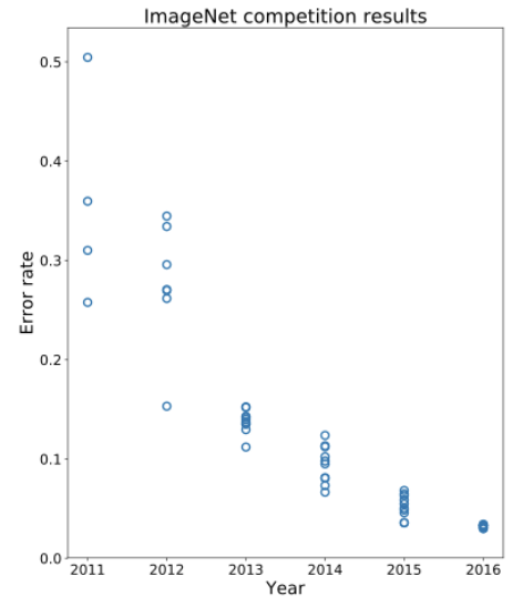
What was responsible for this was a type of machine learning algorithm called a convolutional neural network. Instead of handcrafting the kernels and handcrafting the algorithms for combining the results, this model learns the most useful kernels and the most useful combinations of convolution results!

Has it all been solved?¶

Looking at the graph above, we can see in 2016 we are hitting near human-level performance in these systems. So you might ask: if convolutional neural networks can do a better job classifying images than humans, would they work well for other tasks such as image recognition in self-driving cars?

While these models do very well on the curated training and test data sets, they start behaving very poorly if your data is a little bit different. A pretty shocking example is shown in the image below. Consider the image of the panda on the left, which the model confidently predicts as a panda. But then add a bit of specially-generated noise that is almost imperceptible to the human eye. If you then take this modified image and ask the model to predict the label, the model will even more confidently report that the image depicts something else like a gibbon (a type of ape).

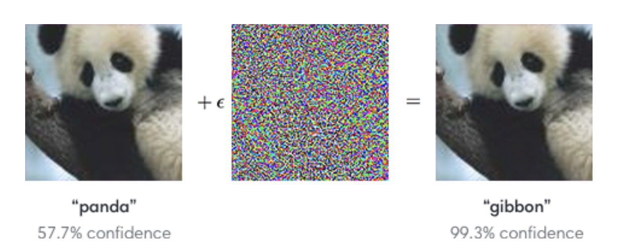
Here are few important ideas to note from this example:

• Even though the picture looks the same to the human eye, the model predicted something completely different.
• Not only did the model make a mistake in this example, but it also very confidently made a mistake!

This should cause us some pause when thinking about using these models in self-driving cars. What if the lighting in the world suddenly changes because it gets cloudy, and now our model now confidently thinks stop signs are green lights?

These adversarial attacks can even be used realistically as patches or stickers. But interestingly, adding noise can also be used for good. A team of researchers at the University of Chicago created a program called Glaze, which adds noise to digital artworks to protect them from being used by generative AI (such as Midjourney, Dall-E, or ChatGPT).

The key insight behind Glaze is that generative AI models learn by studying patterns across thousands or millions of images. If an artist’s work is scraped from the internet and used to train a model, the model can learn to imitate that artist’s style, often without the artist’s knowledge or consent. Glaze works by applying a carefully computed layer of imperceptible noise to an artwork before it is posted online. To the human eye, the image looks unchanged. But to an AI model trying to learn from it, the noise causes the image to appear as if it were in a completely different style, effectively “poisoning” what the model learns.

This is a direct application of the adversarial attack principle from the panda example, but flipped! Instead of fooling a model into making a wrong prediction, Glaze fools a model into learning the wrong thing. Both exploit the same fundamental vulnerability, which is the idea that small, carefully chosen disruptions to pixel values can have an outsized effect on how neural networks process images, even when those disruptions are invisible to humans.

The existence of tools like Glaze raises broader questions worth thinking about:

• Should AI companies be required to disclose what data their models were trained on?
• Is it ethical to train a model on an artist’s work without their permission, even if that work is publicly available online?
• As these tools become more widely used, how might AI companies respond? What does that say about the relationship between AI development and the people whose work it relies on?

There are no easy answers here, and reasonable people disagree. But convolutions and the models built on top of them are increasingly shaping these conversations, which is part of why understanding how they work matters beyond just the code.

⏸️ Pause and 🧠 Think¶

Take a moment to review the following concepts and reflect on your own understanding. A good temperature check for your understanding is asking yourself whether you might be able to explain these concepts to a friend outside of this class.

Here’s what we covered in this lesson:

• numpyfunctions
• axis parameter
• Convolutions
  • Sliding window algorithm
  • Types of kernels
• Convolutional neural networks

Here are some other guiding exercises and questions to help you reflect on what you’ve seen so far:

1. In your own words, write a few sentences summarizing what you learned in this lesson.
2. What did you find challenging in this lesson? Come up with some questions you might ask your peers or the course staff to help you better understand that concept.
3. What was familiar about what you saw in this lesson? How might you relate it to things you have learned before?
4. Throughout the lesson, there were a few Food for thought questions. Try exploring one or more of them and see what you find.

In-Class¶

When you come to class, we will work together on completing convolutions.ipynb! Make sure you have a way of opening and running this file.

Canvas Quiz¶

All done with the lesson? Complete the Canvas Quiz linked here!