Lesson 19. Numpy

The content for this lesson is adapted from material by Hunter Schafer and by Soham Pardeshi.

Objectives¶

By the end of this lesson, students will be able to:

• Apply ndarray arithmetic and logical operators with numbers and other arrays.
• Analyze the shape of an ndarray and index into a multidimensional array.
• Apply arithmetic operators, indexing, and slicing to manipulate RGB images.

Setting up¶

To follow along with the code examples in this lesson, please download the files in the zip folder here:

• lesson19.zip

Make sure to unzip the files after downloading! The following are the main files we will work with:

• lesson19.ipynb
• image_edits.ipynb

NumPy¶

numpy is a Python library for numeric data. Its primary data structure is the array, which stores a sequence of values of the same type. It’s like a pandas.Series, but the index is always integer values like a list.

import numpy as np

# THe function np.array takes a list of alues and returns an ndarray
x = np.array([1, 2, 3, 4])
print(x)

# If there are mixed types, it coerces values to the same type (int -> float)
x = np.array([3.14, 2, 3])
print(x)

The advantage of an ndarray over a built-in Python list is that it’s much more efficient for numeric data processing, especially when there is a very large amount of data. Some example applications include:

• Representing images, where we use a 2-d or 3-d array of pixel brightness values or colors.
• Representing sound or waves, where each point in time represents an amplitude for a frequency
• Scientific computing, such as linear algebra, differential equations, matrix manipulation, and approximation

We have already demonstrated how to create ndarray objects by calling np.array, but there are a few more helpful functions that are used commonly to make an array of any size.

# array initializer takes a list of values
x = np.array([1, 2, 3])
print(x)

# arange is an array-version of the built-in range function
x = np.arange(1, 5)  
print(x)

# ones returns an array storing all 1s of the given length
x = np.ones(5)
print(x)

x = np.zeros(10)
print(x)

Food for thought: When might it be helpful to have an array of 1s, or an array of 0s?

Typing with numpy¶

Typically, when we learn a new library, we use type annotations that refer to both the library and the data type:

• DataFrames are annotated as pd.DataFrame since they come from the pandas library (often abbreviated to pd)
• Graphs are annotated as nx.Graph since they come from the networkx library (often abbreviated to nx)
• GeoDataFrames are annotated as gpd.GeoDataFrame since they come from the geopandas library (often abbreviated to gpd)

However, ndarrays follow a slightly different convention. ndarrays are data structures, and they usually consist of numbers. numpy uses more specific typing than the int or float in base Python, so we have to update our type annotations. To do this, we’ll use the numpy.typing submodule:

import numpy as np
import numpy.typing as npt

def example_function(input: npt.NDArray[np.uint8]) -> npt.NDArray[np.uint8]:
    """
    This function demonstrates type annotations using ndarrays
    """
    return input * 2

Note the following:

• The ndarray is given the annotation npt.NDArray
• uint8 is an integer type specific to numpy and describes the type inside the ndarray
• NDArray is an annotation from numpy.typing, whereas uint8 is an annotation from numpy

Multiple Dimensions¶

It’s possible to make a nested ndarray. Conceptually, we can think of it as a list of lists or other nested data structure that we’ve seen before in Python. Its shape determines the number of dimensions and the size of each dimension. The numpy.ones function actually takes a tuple specifying the shape instead of just a number.

x = np.ones((3, 4))
print(x)

Notice how it prints out as an array of arrays. Since we passed in (3, 4) as the desired shape, it creates an ndarray with 3 rows and 4 columns.

The syntax to access individual elements is very similar to pandas loc. You can even use the “slice” syntax from before to access multiple rows and columns.

x = np.arange(20).reshape((5, 4))
print('x')
print(x)
print()

# Access one value
print('First - x[1, 2]')
print(x[1, 2])
print()

# Access a subset of the values
# Just like with lists/strs, a:b starts at a (inclusive) and goes to b (exclusive)
print('Second - x[2:4, 1:] ')
print(x[2:4, 1:])
print()

# Access an entire row
print('Third - x[3, :]')
print(x[3, :])  # Can also leave off the : at the end (default is :)
print()

# Access an entire column
print('Fourth - x[:, 2]')
print(x[:, 2])

ndarray.shape evaluates to a tuple describing the shape of the array. If it returns (a, b), that means its a 2-d array with a rows and b columns.

x = np.array([0, 1, 2, 3])
print('1-d array with 4 values', x.shape)
print(x)
print('Indexing', x[2])

print()

y = np.array([[0, 1, 2, 3]])
print('2-d array with 1 row, 4 columns', y.shape)
print(y)
print('Indexing', y[0, 2])

print()

z = np.array([[0], [1], [2], [3]])
print('2-d array with 4 rows, 1 column', z.shape)
print(z)
print('Indexing', z[2, 0])

A 2-d ndarray is like a DataFrame. You have to specify a row and a column to get a single value.

A 1-d ndarray is like a Series. You only need to specify the index to get a single value.

ndarray.reshape is a function that takes a target shape tuple and returns a new ndarray with that shape. For example, we can use reshape to change a single-dimension array to one with two dimensions. This will only work if the ndarray.shape has the same number of elements as the target shape.

# Create an array of the values 0 to 20 (exclusive)
x = np.arange(20)
print('Before reshape')
print(x)
print()

# Reshape it so it has dimensions 5x4 (5 rows, 4 columns) 
x = x.reshape((5, 4))
print('After reshape')
print(x)

Arithmetic and Logic¶

Just like pandas, numpy supports element-wise arithmetic and logical operators. We can apply scalar operations to each element in the array:

x = np.arange(4)
print('x')
print(x)
print()

y = x + 3
print('y = x + 3')
print(y)
print()

# Scalar operations also work for arrays with multiple dimensions
m = x.reshape((2, 2))
print('m / 2')
print(m / 2)
print()

We could also apply vector operations between arrays of the same shape. Since the shapes match, operations are applied element-wise. This would work with any mathematical operation (+, -, *, /, //, and **).

z = x + y
print('z = x + y')
print(z)
print()

# Order of operations still applies. Same as (m * 3) + (m / 2)
print('m * 3 + m / 2')
print(m * 3 + m / 2)
print()

You can also use logical operators ==, <, >= to compare ndarray elements. Boolean logic operations like & (and), | (or), and ~ (not) also work as in pandas.

x = np.arange(4)
print('x')
print(x)
print()

# Comparison
print('x < 3')
print(x < 3)
print()

# Using & still requires parentheses
print('(x < 3) & (x % 2 == 0)')
print((x < 3) & (x % 2 == 0))
print()

You can even use masks!

x = np.arange(10)
print('x')
print(x)
print()

mask = (x < 3) & (x % 2 == 0)
print('mask')
print(mask)
print()

y = x[mask]
print('y = x[mask]')
print(y)

Images¶

One of the applications of numpy we discussed earlier was representing image data. In computer science, images are represented as a big 2-d grid of values called pixels. When people talk about screen resolution, they’re really talking about the number of horizontal and vertical pixels on the screen! Each pixel in a greyscale image represents the brightness from black to shades of grey to white.

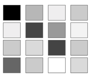
Conventionally, we represent each pixel as a number between 0 and 255. 0 is the darkest value (black) while 255 is the lightest value (white). A grayscale image can be represented as an ndarray of numbers between 0 and 255. Consider the following 4x4 ndarray of pixels:

[[0, 100, 175, 120],
 [180, 61, 83, 130],
 [118, 137, 59, 121],
 [73, 133, 237, 140]]

The 0 in the [0, 0] index would be the darkest value, while the 237 in the [3, 2] index would be the lightest, i.e., closest to white. The other values would be some shade of grey depending on their value. We might visualize the ndarray like the following grid:

At first glance, 255 might seem like an arbitrary number. Where does it come from? It turns out that 255 is the biggest integer that can be stored in a single byte of information. For grayscale images, we typically use one byte to store each pixel in the image. That means saving a grayscale image with ~1000 pixels would take up ~1 kilobyte (i.e. ~1000 bytes) of memory on your computer.

imageio¶

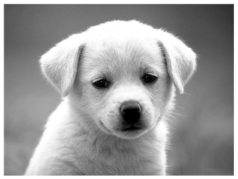
imageio.v3 is a Python library for reading an image to an ndarray. The following code cell reads in an image, prints some values about it, and then plots the image.

import imageio.v3 as iio

# Read in the image
path = 'images/dubs.jpg'
# Use mode='L' to convert to grayscale; mode='P' to preserve colors
dubs = iio.imread(path, mode='L')
# Round the grayscale decimals to integers
dubs = np.uint8(np.rint(dubs))

# Print some values
print('Shape', dubs.shape)
print('Top-left pixel', dubs[0, 0])

# Save it to a file
iio.imwrite('dubs1.png', dubs)

# Modify the numpy array and save that
dubs[-100:, :] = 100

# Save it to a file
iio.imwrite('dubs2.png', dubs)

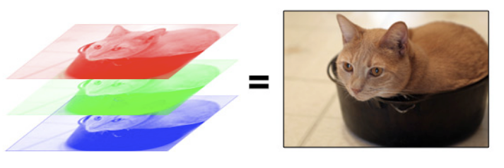
A color image is still represented as an array of pixels except now each pixel has 3 RGB values: a red value, a green value, and a blue value. An RGB image is 3 “grayscale” images stacked on top of each other, but each sub-image corresponds to a particular color channel. Your visual processing system converts the red/blue/green colors to more complex colors such as the cat’s orange/brown shade.

Each pixel will store 3 values between 0 and 255. A color image in numpy will commonly be represented as a 3-dimensional ndarray with shape (height, width, 3). The last dimension has shape 3 because there will be one dimension for each color channel at that pixel location. Visually this makes it kind of like a cube that has “depth” 3 (in the z direction).

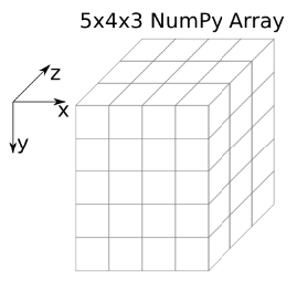
To index into a color image, you now need to specify 3 values such as img[row, col, color], where color is 0 for red, 1 for green, and 2 for blue.

# Read in the image
path = 'images/dubs.jpg'
dubs = iio.imread(path)

# Print some values
print('Shape', dubs.shape)
print('Top-left pixel: Red   =', dubs[0, 0, 0])
print('Top-left pixel: Green =', dubs[0, 0, 1])
print('Top-left pixel: Blue  =', dubs[0, 0, 2])

# Save it to a file
iio.imwrite('dubs.png', dubs)

Now let’s do something slightly more complex where we modify sections of the image. As we modify each section, we are setting one of the red, green, or blue values, respectively.

# Read in the image
path = 'images/dubs.jpg'
dubs = iio.imread(path)

# Remove red from a row of pixels
dubs[100:150, :, 0] = 0

# Remove green from a row of pixels
dubs[200:250, :, 1] = 0

# Make a white column by setting all color channels to 0
dubs[:, 175:200, :] = 255

# Save it to a file
iio.imwrite('dubs.png', dubs)

Broadcasting¶

What happens when the dimensions of two arrays involved in an operation don’t exactly match? Broadcasting is a set of rules numpy uses to evaluate operations with data that disagree in shape. Broadcasting generalizes the rule for evaluating scalar operations such as adding or multiplying to a single number with an array.

You can read more about the full algorithm, but we’ll summarize it here.

When operating on two arrays, numpy compares their shapes element-wise. It starts with the trailing (i.e. rightmost) dimensions and works its way left. Two dimensions are compatible when they are equal, or one of them is 1. When either of the dimensions compared is 1, the other is used. In other words, dimensions with size 1 are stretched or “copied” to match the other.

Arrays do not need to have the same number of dimensions. For example, if you have a 256x256x3 array of RGB values, and you want to scale each color in the image by a different value, you can multiply the image by a one-dimensional array with 3 values. Lining up the sizes of the trailing axes of these arrays according to the broadcast rules, shows that they are compatible:

Image  (3d array): 256 x 256 x 3
Scale  (1d array):             3
Result (3d array): 256 x 256 x 3

Consider the code snippet. We print out the resulting shape and then explain using the rules of broadcasting why this is the case.

m = np.ones((2, 3))  # Shape: (2, 3)
v = np.arange(3)     # Shape: (3,)
result = m + v
print(result)
print(result.shape)

The original values for m and v are ndarrays with different shapes.

m (2, 3)
[[1, 1, 1],
 [1, 1, 1]]

v (3,)
[0, 1, 2]

m is a 2-d array with shape (2, 3) while v is a 2-d array of length 3. m is interpreted as a 2-d array with 2 rows while v is interpreted as a single row.

m (2d array): 2 x 3
v (1d array):     3

Moving from right to left, we note that for the number of columns, 3 matches with 3. But then we note that m has 2 rows while v is missing that dimension entirely. We stretch v along its leftmost dimension (number of rows) so that it has the shape (2, 3).

m (2, 3)
[[1, 1, 1],
 [1, 1, 1]]

v (2, 3)
[[0, 1, 2],
 [0, 1, 2]]

Now, m and v match in their dimensions, so we can apply element-wise arithmetic to them!

⏸️ Pause and 🧠 Think¶

Take a moment to review the following concepts and reflect on your own understanding. A good temperature check for your understanding is asking yourself whether you might be able to explain these concepts to a friend outside of this class.

Here’s what we covered in this lesson:

• numpy
• Creating ndarrays
  • np.arange
  • np.ones
  • np.zeros
• Images in Python
  • imageio
  • 2d images
  • 3d images
• Broadcasting

Here are some other guiding exercises and questions to help you reflect on what you’ve seen so far:

1. In your own words, write a few sentences summarizing what you learned in this lesson.
2. What did you find challenging in this lesson? Come up with some questions you might ask your peers or the course staff to help you better understand that concept.
3. What was familiar about what you saw in this lesson? How might you relate it to things you have learned before?
4. Throughout the lesson, there were a few Food for thought questions. Try exploring one or more of them and see what you find.

In-Class¶

When you come to class, we will work together on completing image_edits.ipynb! Make sure you have a way of opening and running this file.

Canvas Quiz¶

All done with the lesson? Complete the Canvas Quiz linked here!