The content for this lesson is adapted from material by Hunter Schafer.
Objectives
The overall objective for this introduction to machine learning is to provide you with a basic foundation for becoming conversational about machine learning. There’s a lot more that you can study about this topic than what we’ll introduce in this course. This lesson introduces a wholly different model for programming than what we’ve been doing so far, so it’s not unusual to find some of these concepts challenging to learn. By the end of this lesson, students will be able to:
- Describe the difference between traditional algorithms and machine learning algorithms.
- Identify the components of a machine learning model and dataset features and labels.
- Apply
sklearnto train a decision tree for classification and regression tasks.
Setting up
To follow along with the code examples in this lesson, please download the files in the zip folder here:
Make sure to unzip the files after downloading! The following are the main files we will work with:
lesson15.ipynbMLforWeather.ipynbhomes.csvweather.csv
Data Scenarios
Congrats! You have been hired as a data scientist at Bluesky! Your boss comes up to you and tells you that your first task is to answer the age-old question: Which is more popular on the internet, cats or dogs?
Using your CSE 163 knowledge so far, you come up with a good first attempt at trying to answer this question. Your idea is to just scan through all the posts (a list of strings) and just count the number of posts contain the string 'dog' or 'cat'. While this approach doesn’t capture all the complexity of the problem, it is a good starting point for further analysis. You go ahead and write something like the following code.
cats = 0
dogs = 0
for post in posts:
    if 'cat' in post:
        cats += 1
    if 'dog' in post:
        dogs += 1
For str, the in operator scans the post for the substring 'cat' or 'dog' and reports whether the substring is in the post.
Your boss is quite impressed with your work, and now she would like you to solve the same problem using image-based posts instead. You decide to start with what you know and try something similar to what you did with the post data by writing the following code.
cats = 0
dogs = 0
for image in images:
    if cat in image:
        # What's a cat? How do we tell if a cat is in the image?
        cats += 1
    if dog in image:
        # What's a dog? How do we tell if a dog is in the image?
        dogs += 1
Unfortunately, this code only works if the in operator is defined for images. Consider how hard it might be model a cat or a dog in a computer program. Try defining a precise sequence of steps that a computer program can execute to determine, for a given image, whether there is a cat or a dog in the image. It’s tough work!
For reference, an image is defined as a rectangular grid of colored pixels, but it’s never truly the case that a particular pixel’s color definitely corresponds to a cat or a dog. In fact, images can even be of different shapes and sizes, so we can’t even rely on the assumption that we can index a particular pixel in an image.
Machine Learning Overview
Our programming techniques up to this point have focused on specialized algorithms designed to solve problems with a modest model of the underlying phenomena. To answer the question, “What’s the average magnitude of all earthquakes in California?”, our “manual” data analysis for computing the average value of a column in the list of dictionaries format involved defining for loops over the data, defining if conditions with formal logic, and maintaining specialized data structures to keep track of particular totals in only a few columns.
- This algorithm is specialized in that it involved defining a specific, many-step process for computing the particular result. Each time we solve a different problem, we’ll need to write a different algorithm.
- This model is modest in that it involved looking at one or two values per datapoint (row) in the dataset.
For problems where the model is modest, traditional algorithms are ideal since the programmer has total control over the behavior of the program. We can (and have!) answered questions like, “What’s the average magnitude of all earthquakes in California?” using these programming techniques. Data programming libraries like pandas simplify this process by hiding many of the complex algorithmic steps inside DataFrame methods.
In contrast, machine learning (ML) techniques focus on generalized algorithms designed to solve problems with a massive model of the underlying phenomena.
- Machine learning algorithms are generalized in that the same ML algorithm can be applied to a wide range of problems that all fall under the same category.
- Machine learning models are massive in that they involve looking at data with many features—dozens if not hundreds, thousands, or millions of values per datapoint (row) in the dataset.
In our example of classifying cats vs. dogs in images, this would mean a fundamental change to the approach. Rather than attempt to extract a modest model of data from each image (like the color of just a handful of pixels), a machine learning technique would instead let the ML algorithm consider all of the pixels at once to determine patterns or arrangements of pixels that are useful for answering the question. In this way, this task of image recognition in machine learning is inspired by human cognitive faculties: our visual system also works by understanding patterns. Our visual understanding of concepts such as cats, dogs, or faces rely on pattern-based receptive fields.
The machine learning approach to image recognition selects relevant patterns according to training datasets, or datasets of examples for which you already know the answer to your question. Each example consists of a single image (with thousands if not millions of colored pixels) and a label indicating whether the image contains a dog or a cat. The training set is a dataset that you will use to train the model so that it can learn the rules of differentiating between cats and dogs.
A machine learning algorithm (aka “learning algorithm”) takes this training dataset and learns a model that will best predict the label for each example in the training set. In this way, machine learning algorithms are generalized: they can accept any training set and attempt to predict the label given the input image for each example. Whereas labels indicate the expected value for each example in the training set, the features are the inputs to the machine learning algorithm. In the case of an image, we might say that the features are the raw pixel colors for each and every pixel in the image. This is an overwhelming amount of variables for a programmer to work with when writing a traditional algorithm, but not an unusual workload for today’s machine learning algorithms.
Machine learning tasks generally fall into the following categories depending on the data type of the label.
- Regression refers to tasks whose labels are numeric. In this case, models try to produce a “line of best-fit” to accurately predict the label values given some features.
- Classification refers to tasks whose labels are categorical, such as cat vs. dog. In this case, models try to produce a “separator” to classify each example into the expected label category.
Before you begin any machine learning task, ask yourself:
- Do you have a good set of labeled data to train on?
- What features will you use for each example?
- This is sometimes as easy as just including all of the data you have available for each example, but often involves coming up with representations of the data that best help with the prediction task.
- What are the labels that you will try to be learning from?
- What features will you use for each example?
- Is this a regression task or a classification task? What model will you apply for that particular task?
Food for thought: We have yet to bring up the question, “Is this a problem that you can solve in an ethical way using ML?” As you read through the rest of this lesson, consider how the mechanics of how ML models learn might affect when and why we might not want to use it.
Decision Trees
A decision tree is a machine learning model that makes predictions by asking a series of yes/no questions about the features in your data. You can think of a decision tree as an automated way of building a complex chain of if-else statements.
Consider how you might manually write code to predict whether a house is in San Francisco or New York:
if elevation > 50:
    if price > 800000:
        prediction = 'SF'
    else:
        prediction = 'NY'
else:
    if square_feet > 2000:
        prediction = 'NY'
    else:
        prediction = 'SF'
This nested if-else structure is exactly what a decision tree creates! The difference is that instead of you manually deciding which features to check and what threshold values to use (like elevation > 50 or price > 800000), the machine learning algorithm automatically discovers the best questions to ask by analyzing patterns in the training data.
When training a decision tree, the algorithm examines all available features and all possible threshold values to determine which question would be most useful for separating the data. For example, it might consider questions like:
- Is
elevation > 50? - Is
price > 700000? - Is
year_built > 1990? - Is
square_feet > 1500?
The algorithm selects the question that best splits the training examples into groups where each group mostly has the same label. For instance, if asking "Is elevation > 50?" results in one group where 95% of houses are in SF and another group where 90% are in NY, that’s a very useful split!
This splitting process continues recursively. After the first split, the algorithm examines each resulting group and finds the next best question to ask for that subgroup. This creates the tree structure: Each branching point in the tree (called a node) asks a question about one feature, and the answer determines which path to follow down the tree. The tree continues splitting the data until it reaches a leaf node that provides the final prediction for that example.
Using scikit-learn
As with learning data visualization libraries, the objective of this introduction to scikit-learn is to pickup the basic flow of using the library rather than the details of particular functions. We won’t explain every bit of code, nor do we expect you to do so either.
Preparing Data
Consider our example about homes in San Francisco and New York. This dataset has a row for each house, and some various attributes of the house like the city, the house elevation, and the year_built.
Now, let’s load in this dataset and train a machine learning model to predict the city from the other features!
import pandas as pd

data = pd.read_csv('homes.csv')
data.head()
Scikit-learn or sklearn has functions to train and evaluate machine learning models. Like seaborn, sklearn helps us write just a couple lines of code to train an ML algorithm.
In the last section, we introduced two questions we have to ask ourselves when applying an ML task.
- Do you have a good set of labeled data to train on? What are the features? What are the labels?
- Features: All of the columns that describe the house (all but the label
city). - Labels: We want to predict which city a house is in from the features, so
cityis the column that describes that.
- Features: All of the columns that describe the house (all but the label
- Is this a regression task or a classification task? What model will you apply for that particular task?
- This is a classification task since we are predicting SF or NY.
- We haven’t described possible models yet, so we skip this part of the question for now.
So then the first step in training an ML model, is preparing the data so the model can use it.
We start by separating the data into its features and its labels. Notice we are able to also use masking for the columns we want in pandas! This is a succinct way to keep all the columns that aren’t the label we want to predict ('city').
features = data.loc[:, data.columns != 'city']
labels = data['city']
We can then look at the features we will use.
features
Then the labels:
labels
In the cell below, we import a class from sklearn that represents a type of model called a decision tree. The syntax will be reminiscent of what we worked with when we learned about classes and objects.
# Import the model
from sklearn.tree import DecisionTreeClassifier

# Create an untrained model
model = DecisionTreeClassifier()

# Train it on our training data
model.fit(features, labels)
Food for thought: What makes this a classification task?
Using the Model
Now that we have trained the model, we can now use it to make predictions about new examples! We use the predict function on this model to make a prediction for some examples. Since there are nearly 500 houses in this dataset, we make the predictions on a few specified rows and compare the prediction with the label from the original dataset.
predictions = model.predict(features.loc[::80])
print('Predictions:', predictions)
actual_labels = labels.loc[::80]
print('Actual     :', actual_labels.values)  # To get it to print out the same way
That looks pretty good! It looks like it is able to accurately make predictions for those examples (since they match the true labels).
sklearn also provides an function called accuracy_score to evaluate how well a model is doing on some dataset. This only works for classification problems, and it returns the percentage of examples the model predicted correctly! You give it both the true labels and the predicted labels, and it computes this accuracy score for you. Accuracy scores will be any number between:
- 0, meaning your model predicted 0% of the labels correctly
- 1.0, meaning your model correctly predicted all labels
from sklearn.metrics import accuracy_score

predictions = model.predict(features)
accuracy_score(labels, predictions)
🎉 We are able to get 100% of the examples correct! 🎉 But as the last reading hinted at, this might not be indicative that our tree will have 100% accuracy on future data… It turns out that evaluating an ML model is an entire subfield of computing, and the reality is that this model won’t always work as well as it does on our training set. We’ll discuss in the next lesson how to better evaluate this model.
Visualizing the Model
Finally, we will quickly show that sklearn provides a way of visualizing the decision tree! The code is a little complex, and this is something taken from their documentation. Note that you might not be able to view the whole tree in the notebook!
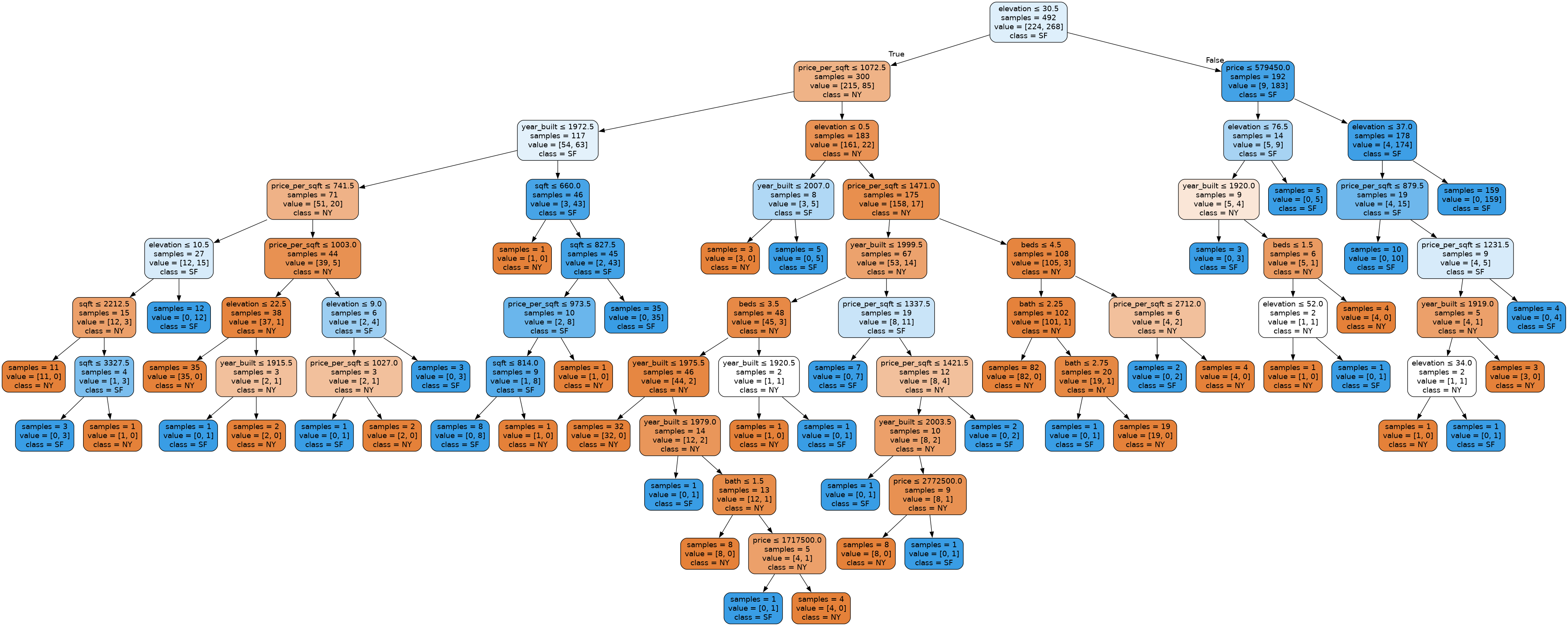
from IPython.display import Image, display

import graphviz
from sklearn.tree import export_graphviz


def plot_tree(model, features, labels):
    dot_data = export_graphviz(model, out_file=None,
            feature_names=features.columns,
            class_names=labels.unique(),
            impurity=False,
            filled=True, rounded=True,
            special_characters=True)
    graphviz.Source(dot_data).render('tree.gv', format='png')
    display(Image(filename='/home/tree.gv.png'))


plot_tree(model, features, labels)
Recap
We introduced a lot of new concepts and code fragments on this slide. For a quick recap, here are all the “important” bits to train an ML model for this task.
# Import pandas
import pandas as pd
# Import the model
from sklearn.tree import DecisionTreeClassifier
# Import the function to compute accuracy
from sklearn.metrics import accuracy_score

# Read in data
data = pd.read_csv('homes.csv')

# Separate data into features and labels
features = data.loc[:, data.columns != 'city']
labels = data['city']

# Create an untrained model
model = DecisionTreeClassifier()
# Train it on our training data
model.fit(features, labels)

# Make predictions on the data
predictions = model.predict(features)
# Assess the accuracy of the model
accuracy_score(labels, predictions)
⏸️ Pause and 🧠 Think
Take a moment to review the following concepts and reflect on your own understanding. A good temperature check for your understanding is asking yourself whether you might be able to explain these concepts to a friend outside of this class.
Here’s what we covered in this lesson:
- Machine learning terminology
- Decision trees
- Machine learning algorithms
- Training data
- Examples
- Features
- Labels
- Regression
- Classification
Here are some other guiding exercises and questions to help you reflect on what you’ve seen so far:
- In your own words, write a few sentences summarizing what you learned in this lesson.
- What did you find challenging in this lesson? Come up with some questions you might ask your peers or the course staff to help you better understand that concept.
- What was familiar about what you saw in this lesson? How might you relate it to things you have learned before?
- Throughout the lesson, there were a few Food for thought questions. Try exploring one or more of them and see what you find.
In-Class
When you come to class, we will work together on answering some conceptual questions and completing MLforWeather.ipynb! Make sure you have a way of opening and running this file.
Canvas Quiz
All done with the lesson? Complete the Canvas Quiz linked here!