Model Evaluation
In this lesson, we'll learn how to evaluate the quality of a machine learning model. By the end of this lesson, students will be able to:
- Apply
get_dummiesto represent categorical features as one or more dummy variables. - Apply
train_test_splitto randomly split a dataset into a training set and test set. - Evaluate machine learning models in terms of overfit and underfit.
from sklearn.linear_model import LinearRegression
from sklearn.metrics import mean_squared_error

import pandas as pd
Dummy variables
Last time, we tried to predict the price of a home from all the other variables. However, we learned that since the city column contains categorical string values, we can't use it as a feature in a regression algorithm.
homes = pd.read_csv("homes.csv")
homes
| beds | bath | price | year_built | sqft | price_per_sqft | elevation | city | |
|---|---|---|---|---|---|---|---|---|
| 0 | 2.0 | 1.0 | 999000 | 1960 | 1000 | 999 | 10 | NY |
| 1 | 2.0 | 2.0 | 2750000 | 2006 | 1418 | 1939 | 0 | NY |
| 2 | 2.0 | 2.0 | 1350000 | 1900 | 2150 | 628 | 9 | NY |
| 3 | 1.0 | 1.0 | 629000 | 1903 | 500 | 1258 | 9 | NY |
| 4 | 0.0 | 1.0 | 439000 | 1930 | 500 | 878 | 10 | NY |
| ... | ... | ... | ... | ... | ... | ... | ... | ... |
| 487 | 5.0 | 2.5 | 1800000 | 1890 | 3073 | 586 | 76 | SF |
| 488 | 2.0 | 1.0 | 695000 | 1923 | 1045 | 665 | 106 | SF |
| 489 | 3.0 | 2.0 | 1650000 | 1922 | 1483 | 1113 | 106 | SF |
| 490 | 1.0 | 1.0 | 649000 | 1983 | 850 | 764 | 163 | SF |
| 491 | 3.0 | 2.0 | 995000 | 1956 | 1305 | 762 | 216 | SF |
492 rows × 8 columns
This problem not only occurs when using DecisionTreeRegressor, but it also occurs when using LinearRegression since we can't multiply a categorical string value with a numeric slope value. Let's learn how to represent these categorical features as one or more dummy variables.
def model_parameters(reg, columns):
    """Returns a string with the linear regression model parameters for the given column names."""
    slopes = [f"{coef:.2f}({columns[i]})" for i, coef in enumerate(reg.coef_)]
    return " + ".join([f"{reg.intercept_:.2f}"] + slopes)
pd.get_dummies(X)
---------------------------------------------------------------------------
NameError                                 Traceback (most recent call last)
Cell In[4], line 1
----> 1 pd.get_dummies(X)

NameError: name 'X' is not defined
# In the design space of how I setup my problem, I can get dummy variables for categorical variables
# I can remove certain variables
# I can add interaction effects
X = pd.get_dummies(homes[["beds", "bath", "year_built", "sqft", "price_per_sqft", "elevation", "city"]])
y = homes["price"]
# "NY" can get its own slope versus "SF"
# Or, "NY" could have the opposite (negative) slope of "SF"
reg = LinearRegression().fit(X, y)

print("Model:", model_parameters(reg, X.columns))
print("Error:", mean_squared_error(y, reg.predict(X)))
# Interaction effect
X["interaction"] = X["sqft"] * X["price_per_sqft"]
X
reg = LinearRegression().fit(X, y)

print("Model:", model_parameters(reg, X.columns))
print("Error:", mean_squared_error(y, reg.predict(X)))
y
---------------------------------------------------------------------------
NameError                                 Traceback (most recent call last)
Cell In[5], line 1
----> 1 y

NameError: name 'y' is not defined
Overfitting
In our introduction to machine learning, we explained that the researchers who worked on calibrating PurpleAir Sensor (PAS) measurements against the EPA Air Quality Sensor (AQS) measurements ultimately decided to use the model that included only the PAS and humidity features (variables)—ignoring the opportunity to use the temperature and dew point even though a model that includes all features produced a lower overall mean squared error.
sensor_data = pd.read_csv("sensor_data.csv")
sensor_data
| AQS | temp | humidity | dew | PAS | |
|---|---|---|---|---|---|
| 0 | 6.7 | 18.027263 | 38.564815 | 3.629662 | 8.616954 |
| 1 | 3.8 | 16.115280 | 49.404315 | 5.442318 | 3.493916 |
| 2 | 4.0 | 19.897634 | 29.972222 | 1.734051 | 3.799601 |
| 3 | 4.7 | 21.378334 | 32.474513 | 4.165624 | 4.369691 |
| 4 | 3.2 | 18.443822 | 43.898226 | 5.867611 | 3.191071 |
| ... | ... | ... | ... | ... | ... |
| 12092 | 5.5 | -12.101337 | 54.188889 | -19.555834 | 2.386120 |
| 12093 | 16.8 | 4.159967 | 56.256030 | -3.870659 | 32.444987 |
| 12094 | 15.6 | 1.707895 | 65.779221 | -4.083768 | 25.297018 |
| 12095 | 14.0 | -14.380144 | 48.206481 | -23.015378 | 8.213208 |
| 12096 | 5.8 | 5.081813 | 52.200000 | -4.016401 | 9.436011 |
12097 rows × 5 columns
from sklearn.metrics import root_mean_squared_error

X = sensor_data[["AQS", "temp", "humidity", "dew"]]
y = sensor_data["PAS"]
reg = LinearRegression().fit(X, y)

print("Model:", model_parameters(reg, X.columns))
# RMSE, or root mean squared error, is the square root of the mean of the squared errors.
print("Error:", root_mean_squared_error(y, reg.predict(X)))
Model: -11.57 + 1.91(AQS) + 0.02(temp) + 0.17(humidity) + -0.04(dew)
Error: 4.797814359357567
In fact, the authors (Barkjohn et al. 2021) tested the impact of incrementally introducing a feature to the model to determine which combination of features could provide the most useful model—not necessarily the most accurate one. Their research additionally included interactions between features indicated by the × symbol. For each grouping of models with a certain number of features, they highlighted the model with the lowest root mean squared error (RMSE, or the square root of the MSE) using an asterisk *.
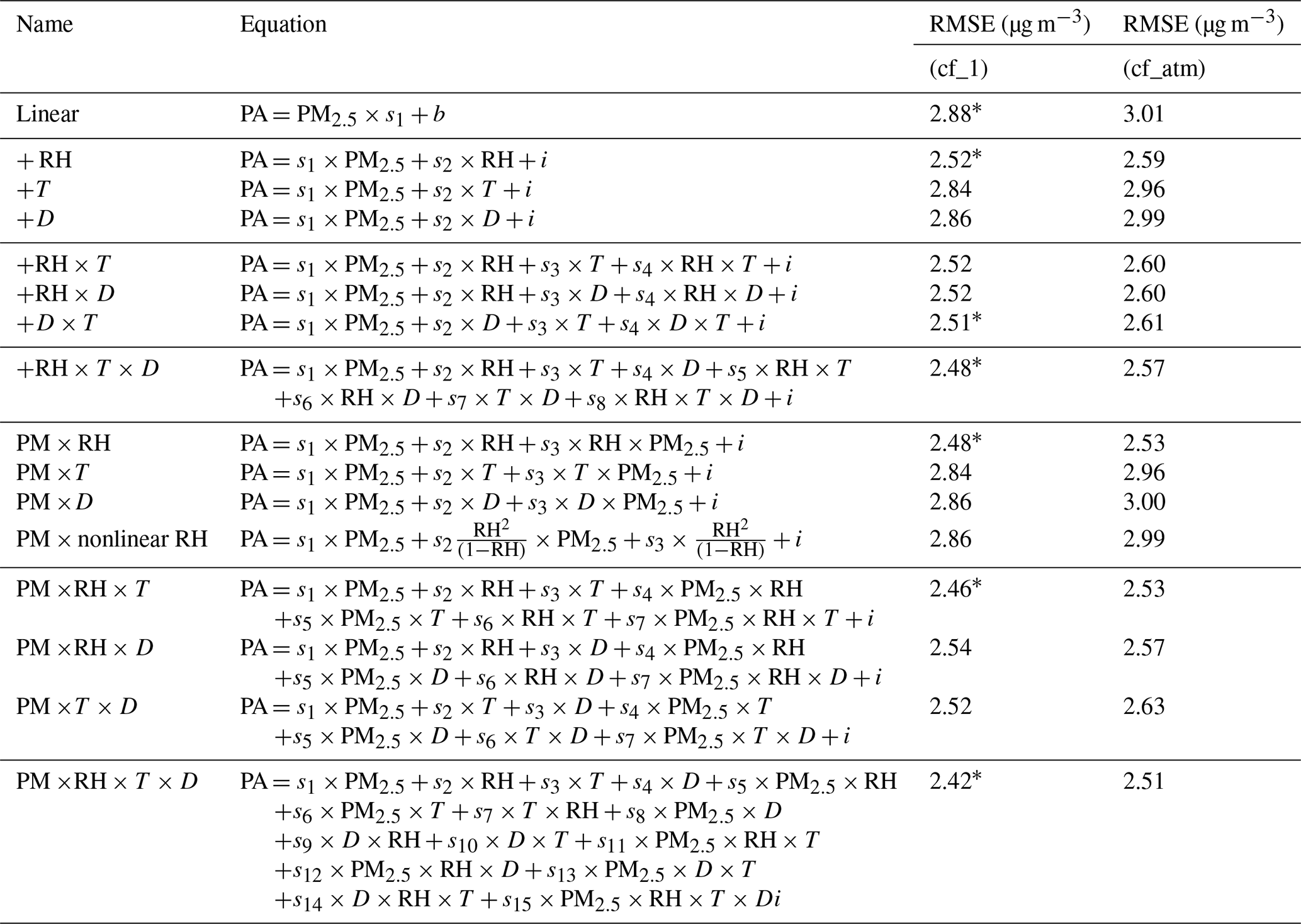
The model at the bottom of the table that includes all the features also has the lowest RMSE loss. But the loss value alone is not a convincing measure: adding more features into a model not only leads to a model that is harder to explain, but also increases the possibility of overfitting.
A model is considered overfit if its predictions correspond too closely to the training dataset such that improvements reported on the training dataset are not reflected when the model is run on a testing dataset (or in the real world). To simulate training and testing datasets, we can take our X features and y labels and subdivide them into X_train, X_test, y_train, y_test using the train_test_split function. The testing dataset should only be used during final model evaluation when we're ready to report the overall effectiveness of our final machine learning model.
from sklearn.model_selection import train_test_split
from sklearn.tree import DecisionTreeRegressor

# test_size=0.2 indicates 80% training dataset and 20% testing dataset
# train_test_split shuffles your data
# Doing a train-test split is part of holding-out your data
X_train, X_test, y_train, y_test = train_test_split(X, y, test_size=0.2)

# During model training, use only the training dataset
# Here, when no max_depth is specified, there is no limit
reg = DecisionTreeRegressor().fit(X_train, y_train)

# print("Model:", model_parameters(reg, X_train.columns))
print("Error:", root_mean_squared_error(y_test, reg.predict(X_test)))
Error: 5.426843608165562
Feature selection
Feature selection describes the process of selecting only a subset of features in order to improve the quality of a machine learning model. In the air quality sensor calibration study, we can begin with all the features and gradually remove the least-important features one-by-one.
features = ["AQS", "humidity", "temp", "dew"]

reg = LinearRegression().fit(X_train.loc[:, features], y_train)
print("Model:", model_parameters(reg, features))
print("Error:", root_mean_squared_error(y_test, reg.predict(X_test.loc[:, features])))
Model: -11.56 + 1.92(AQS) + 0.17(humidity) + 0.01(temp) + -0.04(dew)
Error: 4.7693574628022954
Recursive feature elimination (RFE) automates this process by starting with a model that includes all the variables and removes features from the model starting with the ones that contribute the least weight (smallest coefficients in a linear regression).
from sklearn.feature_selection import RFE

# Remove 1 feature per step until half the original features remain
rfe = RFE(LinearRegression(), step=1, n_features_to_select=0.75, verbose=1)
rfe.fit(X_train, y_train)

# Show the final subset of features
rfe_features = X.columns[[r == 1 for r in rfe.ranking_]]
print("Features:", list(rfe_features))

# Extract the last LinearRegression model trained on the final subset of features
reg = rfe.estimator_

print("Model:", model_parameters(reg, rfe_features))
print("Error:", root_mean_squared_error(y_test, rfe.predict(X_test)))
Fitting estimator with 4 features.
Features: ['AQS', 'humidity', 'dew']
Model: -11.11 + 1.92(AQS) + 0.17(humidity) + -0.02(dew)
Error: 4.7695778136648705
Cross validation
How do we know when to stop removing features during feature selection? We can certainly use intuition or look at the changes in error as we remove each feature. But this still requires us to evaluate the model somehow. If the testing dataset can only be used at the end of model evaluation, it was wrong of us to use the testing dataset during feature selection!
Cross-validation provides one way to help us explore different models before we choose a final model for evaluation at the end. Cross-validation lets us evaluate models without touching the testing dataset by introducing new validation datasets.
The simplest way to cross-validate is to call the cross_val_score helper function on an unfitted machine learning algorithm and the dataset. This function will further subdivide the training dataset into 5 folds and, for each of the 5 folds, train a separate model on the training folds and evaluate them on the validation fold.

The scoring parameter can accept the string name of a scorer function. Higher (more positive) scores are considered better, so we use the negative RMSE value as the scorer function.
from sklearn.model_selection import cross_val_score
from sklearn.tree import DecisionTreeRegressor

cross_val_score(
    estimator=DecisionTreeRegressor(max_depth=7),
    X=X_train,
    y=y_train,
    scoring="neg_root_mean_squared_error",
    verbose=3,
).mean()
[CV] END ............................... score: (test=-5.173) total time=   0.0s
[CV] END ............................... score: (test=-4.606) total time=   0.0s
[CV] END ............................... score: (test=-5.660) total time=   0.0s
[CV] END ............................... score: (test=-4.416) total time=   0.0s
[CV] END ............................... score: (test=-4.682) total time=   0.0s
-4.907376955650832
As we've seen throughout these lessons on machine learning, we prefer to automate our processes. Rather than modify the max_depth and manually tweaking the values until we find something that works, we can use GridSearchCV to exhaustively search all hyperparameter options. Here, the first 5 folds for max_depth=2 are exactly the same as cross_val_score.
from sklearn.model_selection import GridSearchCV

search = GridSearchCV(
    estimator=DecisionTreeRegressor(),
    param_grid={
        "max_depth": [2, 3, 4, 5, 6, 7, 8, 9, 10]
    },
    scoring="neg_root_mean_squared_error",
    verbose=3,
)
search.fit(X_train, y_train)

# Show the best score and best estimator at the end of hyperparameter search
print("Mean score for best model:", search.best_score_)
reg = search.best_estimator_
print("Best model:", reg)
Fitting 5 folds for each of 9 candidates, totalling 45 fits
[CV 1/5] END ......................max_depth=2;, score=-6.637 total time=   0.0s
[CV 2/5] END ......................max_depth=2;, score=-5.824 total time=   0.0s
[CV 3/5] END ......................max_depth=2;, score=-7.973 total time=   0.0s
[CV 4/5] END ......................max_depth=2;, score=-5.966 total time=   0.0s
[CV 5/5] END ......................max_depth=2;, score=-6.485 total time=   0.0s
[CV 1/5] END ......................max_depth=3;, score=-6.254 total time=   0.0s
[CV 2/5] END ......................max_depth=3;, score=-5.674 total time=   0.0s
[CV 3/5] END ......................max_depth=3;, score=-7.273 total time=   0.0s
[CV 4/5] END ......................max_depth=3;, score=-5.429 total time=   0.0s
[CV 5/5] END ......................max_depth=3;, score=-6.011 total time=   0.0s
[CV 1/5] END ......................max_depth=4;, score=-5.761 total time=   0.0s
[CV 2/5] END ......................max_depth=4;, score=-4.918 total time=   0.0s
[CV 3/5] END ......................max_depth=4;, score=-6.146 total time=   0.0s
[CV 4/5] END ......................max_depth=4;, score=-4.850 total time=   0.0s
[CV 5/5] END ......................max_depth=4;, score=-5.542 total time=   0.0s
[CV 1/5] END ......................max_depth=5;, score=-5.356 total time=   0.0s
[CV 2/5] END ......................max_depth=5;, score=-4.767 total time=   0.0s
[CV 3/5] END ......................max_depth=5;, score=-5.860 total time=   0.0s
[CV 4/5] END ......................max_depth=5;, score=-4.664 total time=   0.0s
[CV 5/5] END ......................max_depth=5;, score=-5.139 total time=   0.0s
[CV 1/5] END ......................max_depth=6;, score=-5.226 total time=   0.0s
[CV 2/5] END ......................max_depth=6;, score=-4.757 total time=   0.0s
[CV 3/5] END ......................max_depth=6;, score=-5.756 total time=   0.0s
[CV 4/5] END ......................max_depth=6;, score=-4.480 total time=   0.0s
[CV 5/5] END ......................max_depth=6;, score=-4.788 total time=   0.0s
[CV 1/5] END ......................max_depth=7;, score=-5.173 total time=   0.0s
[CV 2/5] END ......................max_depth=7;, score=-4.606 total time=   0.0s
[CV 3/5] END ......................max_depth=7;, score=-5.660 total time=   0.0s
[CV 4/5] END ......................max_depth=7;, score=-4.416 total time=   0.0s
[CV 5/5] END ......................max_depth=7;, score=-4.710 total time=   0.0s
[CV 1/5] END ......................max_depth=8;, score=-4.916 total time=   0.0s
[CV 2/5] END ......................max_depth=8;, score=-6.268 total time=   0.0s
[CV 3/5] END ......................max_depth=8;, score=-5.763 total time=   0.0s
[CV 4/5] END ......................max_depth=8;, score=-4.476 total time=   0.0s
[CV 5/5] END ......................max_depth=8;, score=-4.732 total time=   0.0s
[CV 1/5] END ......................max_depth=9;, score=-5.007 total time=   0.0s
[CV 2/5] END ......................max_depth=9;, score=-4.667 total time=   0.1s
[CV 3/5] END ......................max_depth=9;, score=-5.743 total time=   0.1s
[CV 4/5] END ......................max_depth=9;, score=-4.473 total time=   0.1s
[CV 5/5] END ......................max_depth=9;, score=-5.139 total time=   0.0s
[CV 1/5] END .....................max_depth=10;, score=-4.974 total time=   0.1s
[CV 2/5] END .....................max_depth=10;, score=-6.452 total time=   0.0s
[CV 3/5] END .....................max_depth=10;, score=-5.936 total time=   0.1s
[CV 4/5] END .....................max_depth=10;, score=-4.701 total time=   0.1s
[CV 5/5] END .....................max_depth=10;, score=-5.114 total time=   0.1s
Mean score for best model: -4.912978616272581
Best model: DecisionTreeRegressor(max_depth=7)
Finally, we can report the test error for the best model by evaluating it against the testing dataset. Why is the testing dataset error different from the mean score for the best model printed above?
print("Error:", root_mean_squared_error(y_test, reg.predict(X_test)))
Error: 4.783060341092756
Visualizing decision tree models
Last time, we plotted the predictions for a linear regression model that was trained to take AQS measurements and predict PAS measurements. What do you think a decision tree model would look like for this simplified PurpleAir sensor calibration problem?
Here's a complete workflow for decision tree model evaluation using the practices above. The resulting plot compares a linear regression model lmplot against the decisions made by a decision tree.
X_demo
| AQS | |
|---|---|
| 0 | 0.0 |
| 1 | 1.0 |
| 2 | 2.0 |
| 3 | 3.0 |
| 4 | 4.0 |
| ... | ... |
| 104 | 104.0 |
| 105 | 105.0 |
| 106 | 106.0 |
| 107 | 107.0 |
| 108 | 108.0 |
109 rows × 1 columns
X = sensor_data[["AQS", "temp", "humidity", "dew"]]
y = sensor_data["PAS"]

# Re-split dataset into 80% training dataset and 20% testing dataset
X_train, X_test, y_train, y_test = train_test_split(X, y, test_size=0.2)

# Recursive feature elimination to select the single most important feature based on slope value
rfe = RFE(LinearRegression(), n_features_to_select=1)
rfe.fit(X_train, y_train)
# Identify the best feature to predict PAS
rfe_feature = X.columns[rfe.ranking_.argmin()]
# Use only the best feature (AQS)
X = X[[rfe_feature]]
X_train = X_train[[rfe_feature]]
X_test = X_test[[rfe_feature]]

# Grid search cross-validation to tune the max_depth hyperparameter using RMSE loss metric
search = GridSearchCV(
    estimator=DecisionTreeRegressor(),
    param_grid={"max_depth": [2, 3, 4, 5, 6, 7, 8, 9, 10]},
    scoring="neg_root_mean_squared_error"
)
search.fit(X_train, y_train)
reg = search.best_estimator_

# Visualize the LinearRegression model (lmplot)
import matplotlib.pyplot as plt
import numpy as np
import seaborn as sns
from sklearn.tree import plot_tree
sns.set_theme()
sns.lmplot(sensor_data, x=rfe_feature, y="PAS").set(title="Linear regression for PAS")

# Compare the results to the decision tree outputs by plotting the points from 0 to the max PAS value
grid = sns.relplot(sensor_data, x=rfe_feature, y="PAS").set(title="Decision tree regressor for PAS")
# arange sets up a list of numbers from 0 to the max AQS value
X_demo = pd.DataFrame(np.arange(X[rfe_feature].max()), columns=[rfe_feature])
# Pick out the main plot (there's only one plot),
# then plot a line from all the X_demo points to the predictions produced by the decision tree
# Here, the plot function is a matplotlib
grid.facet_axis(0, 0).plot(X_demo, reg.predict(X_demo))

# Show nodes in the decision tree
plt.figure(dpi=300)
plot_tree(
    reg,
    max_depth=2, # Only show the first two levels
    feature_names=[rfe_feature],
    label="root",
    filled=True,
    impurity=False,
    proportion=True,
    rounded=False
);


reg.predict(X_demo)
array([  2.77001316,   2.77001316,   2.77001316,   3.51526378,
         4.62700979,   6.12715305,   7.71307412,   9.7356668 ,
        11.94350969,  13.8986451 ,  15.69696189,  17.54030683,
        19.67781562,  22.37804526,  25.34833327,  27.32645843,
        27.32645843,  34.26822128,  34.26822128,  34.26822128,
        39.2305876 ,  39.2305876 ,  39.2305876 ,  39.2305876 ,
        39.2305876 ,  48.89468561,  48.89468561,  48.89468561,
        48.89468561,  48.89468561,  48.89468561,  48.89468561,
        48.89468561,  48.89468561,  48.89468561,  48.89468561,
        68.15333007,  68.15333007,  68.15333007,  68.15333007,
        68.15333007,  68.15333007,  68.15333007,  68.15333007,
        68.15333007,  68.15333007,  68.15333007,  68.15333007,
        68.15333007,  68.15333007, 114.23413889, 114.23413889,
       114.23413889, 114.23413889, 114.23413889, 114.23413889,
       128.60872569, 128.60872569, 128.60872569, 128.60872569,
       128.60872569, 128.60872569, 128.60872569, 128.60872569,
       128.60872569, 128.60872569, 128.60872569, 128.60872569,
       128.60872569, 128.60872569, 128.60872569, 128.60872569,
       128.60872569, 128.60872569, 128.60872569, 128.60872569,
       128.60872569, 128.60872569, 128.60872569, 128.60872569,
       128.60872569, 128.60872569, 128.60872569, 128.60872569,
       128.60872569, 256.30960922, 256.30960922, 256.30960922,
       256.30960922, 256.30960922, 256.30960922, 256.30960922,
       256.30960922, 256.30960922, 256.30960922, 256.30960922,
       256.30960922, 256.30960922, 256.30960922, 256.30960922,
       256.30960922, 256.30960922, 256.30960922, 256.30960922,
       256.30960922, 256.30960922, 256.30960922, 256.30960922,
       256.30960922])
The testing dataset error rates for both the DecisionTreeRegressor and the LinearRegression models are not too far apart. Which model would you prefer to use? Justify your answer using either the error rates below or the visualizations above.
print("Tree error:", root_mean_squared_error(y_test, search.predict(X_test)))
print("Line error:", root_mean_squared_error(
    y_test,
    LinearRegression().fit(X_train, y_train).predict(X_test),
))
Tree error: 5.3645462062990905
Line error: 5.395609694450481
Earlier, we discussed how overfitting to the testing dataset can be mitigated by using cross-validation. But in answering the previous question on whether we should prefer a DecisionTreeRegressor model or a LinearRegression model, we've actually overfit the model by hand! Explain how preferring one model over the other according to the visualization overfits to the testing dataset.