Programming

Useful CSE 160 Resources¶

• CSE 160 Code Quality Guide
• flake8 References

Learning Objectives¶

In this assignment you will:

• Write a full Python program from scratch and without a starting template
• Read and process data from a given comma-separated values (CSV) file
• Build and handle a highly nested structure
• Create plots and graphs to visualize different aspects of the data
• Write tests to ensure the validity of your program
• Practice good coding styles, as defined by the course style guide

Introduction¶

Fish is a major source of protein and nutrition around the world. As our population grows, so does our fish consumption and the industry of farming and catching fish must grow to match. In this assignment, you will write a Python program to analyze data from the United Nations Food and Agriculture Organization.

For many of the problems below, you will be asked to write short answers for a couple of questions. Put these answers into the answers.txt file provided.

Problem 0: Setting up and Program Organization¶

1. Download and extract homework6.zip
2. You should have a folder with four files:
   1. fishing.py - a file where you will write your code; this includes the function headers for all the functions we will ask you to write, plus a few given helper functions that should not be modified
   2. fishing_tests.py - a nearly-empty file where you will write your tests
   3. small.csv - a small subset of the data that you should use for testing
   4. large.csv - the full, larger set of data that you will use for answering the final questions
3. Make sure you have all of these files in the same folder. The subsequent problems and questions will explain in further detail the format and expected usage of the data.

In this assignment you will be asked to write the following functions; all of which will be expected and run by the autograder. We have provided function headers for all of the expected function. You are expected to implement all of them as defined in this specification.

• parse_data(filename)
• get_actual_production(data)
• get_production_need(data)
• plot_production_vs_consumption(data, country_code)
• predict_need(production_need, predict_years)
• total_production_need(data, years_to_predict)

The development pattern for this assignment is similar to past assignments. You will start by writing a function to read data from a file. Then, pass that data (i.e., the return value from parse_data) into a series of helper functions that will transform that data and perform useful calculations. Along the way, we will ask you guiding questions and ask you to plot some of the data.

Problem 1: Read in the data¶

The smaller data file, small.csv, contains production (both wild and farmed), consumption, and population data for three countries for a small number of years.

For this problem, you will write a function that parses the input file as a CSV file, and returns a dictionary containing the data for each country in the file.

The input files have the following format:

country code,full name,measure (wild caught, farmed, consumption, or population),1950,1951,1952,...

There will always be at minimum three fields for each row: Every line will have at minimum a country code, full country name, and which measure this row is for. There will be the proper number of commas to represent every year, but not all years are guaranteed to have values. For example, the following is an example file containing the header row and four data rows:

country,country code,measure,1960,1961
Ankh-Morpork,AMP,consumption,,10.42
Ankh-Morpork,AMP,wild caught,7777,8888
Ankh-Morpork,AMP,farmed,321,333
Ankh-Morpork,AMP,population,995623,996235

Pre-coding questions:¶

Before writing code for this assignment, answer the following questions in the answer.txt file. You may find it helpful in answering the questions to read the entire assignment specification first. These are meant to help you better understand the structure of the data and how to parse it from the CSV.

1. Why are there multiple rows for Ankh-Morpork? Why isn’t there just a single row for this country?
2. What do you notice about the data for 1960? How do you think that affects how you’ll handle reading the data in this problem’s functions? (Hint: read the tip above.)
3. The consumption measurement type is clearly labeled (line 2 of the file), but none of the other lines are labeled “production”. If you were to ask “how much seafood did Ankh-Morpork produce in 1960?” how would you come up with the answer? (Hint: the answer would be 8098.)

parse_data(filename):¶

For this problem, write a function called parse_data(filename) in the fishing.py file that reads the data in filename, parsing as a CSV, and returning a dictionary containing the data for each country in the file.

Given the example CSV shown earlier in Problem 1, the dictionary returned from parse_data would look like the following:

{
    "min_year": 1960,
    "max_year": 1961,
    "farmed": {
        "AMP": {1960: 321, 1961: 333},
    },
    "wild caught": {
        "AMP": {1960: 7777, 1961: 8888},
    },
    "consumption": {
        "AMP": {1960: None, 1961: 10.42},
    },
    "population": {
        "AMP": {1960: 995623, 1961: 996235},
    },
}

This is a triply nested dictionary; that is, a dictionary with values as dictionaries where those values are also dictionaries. From outside in, the structure of the dictionary is as follows:

For the outermost dictionary:

• The keys are the four different types of measurements: farmed, wild caught, consumption, and population.
• The values are dictionaries representing the data for that specific measure.

For the second-level dictionary, for example the value of the 'farmed' key from the outmost dictionary:

• The keys are the three-letter country codes represented in the data. For example, “AMP”, “USA”, “MEX”, etc. These match the "country code" column from the CSV files.
• The values are dictionaries, representing the data specific to the key (i.e., country) for the measure it’s nested within.

For the innermost dictionary:

• The keys are the years represented in the data. (E.g., 1960, 1961) These should be integers.
• The values are the measurements for that year or None if there is no data for that year (represented as empty string ('') from csv.DictReader). The types for these values should be as follows:
  • farmed, wild caught, and consumption should all be floats
  • population should be an integer

Consider as an example a subset of the above example dictionary: { "farmed": { "AMP": {1960: 321, 1961: 333} } }. Reading this from the inside out we would say that in 1961, the country “AMP” had farmed 333 metric tonnes of fish.

You should use the min_year and max_year functions provided to you in the starter files to get the range of years for which data is available. If you’ve created a csv.DictReader as reader = csv.DictReader(file) then you can set the min and max years like data["min_year"] = min_year(reader.fieldnames).

Problem 2: How many can we feed?¶

A straightforward way to determine if a country is producing enough seafood for its citizens is to see how many people could be fed given the consumption and production rates. The unit of measurement for the consumption data in this assignment is kg per capita per year (that is, in the given year how many kilograms of seafood, on average, did each resident of that country eat). And, the units for production data is given in metric tons (1000kg).

To calculate if there’s enough production, we’ll need to combine and modify some of the data.

Problem 2a: get_actual_production¶

For this problem, write a function called get_actual_production(data, country_code, year) that returns the actual production for a given country and year, using data as produced by Problem 1’s parse_data. This value should be the sum of the farmed and wild caught values for that country for that year. For example, given the sample data shown in Problem 1, calling get_actual_production(data, "AMP", 1960) should return 8098.

The following should be considered for handling missing data points:

• If both farmed and wild caught are missing for the given year and country, then the function should return None.
• If only one of farmed or wild caught is missing for the given year and country, then the function should return the other value.

Problem 2b: get_production_need¶

For this problem, write a function called get_production_need(data, country_code, year) that returns the amount of seafood production that is needed to feed the country’s population for the given year, using data as produced by Problem 1’s parse_data. The consumption values in the data are specified as kilograms / capita / year. Since the production values are given in metric tons (1000kg), we will need to convert the consumption values to metric tons.

We can therefore calculate the necessary production with:

$\text{production need} = \frac{\text{population} \times \text{consumption}}{1000}$

For example, using the sample data shown in Problem 1, calling get_production_need(data, "AMP", 1961) should return 10380.76 (your precision may vary).

If either population or consumption is missing for the given year and country, then the function should return None.

Problem 2c: Adding Tests¶

In the fishing_tests.py file, write a function called test_get_production_need() that runs two distinctly different tests for the get_production_need function. These tests should be written in the form:

assert actual_int == expected_int
assert math.isclose(actual_float, expected_float)

You may find it helpful to start with the example data given in this specification.

For this problem (2c), you will be graded primarily on one criteria: are the two test cases you come up with meaningfully different? Refer to the lecture on Testing for discussion on what constitutes “meaningfully different.”

Note that you are not being asked to write tests for the get_actual_production function. However you may find it helpful to do so. If you do, write those tests in a different function.

Some tips for designing and writing your tests:

• We have not provided tests or exact results to check your program against. We require you to write your own tests and to use assert statements.
  • You can and should refer to past assignments (Homework 4 is a good example) to see how to write and structure your tests.
• We HIGHLY encourage you to write tests before writing the functions. Doing so will allow you to check your work as you write your functions and ensure that you catch more bugs in your code.
• You do not need to test functions that generate plots or print output. Additionally, you do not need to create extra data files for testing, although you are welcome to do so to improve your test suite. However, since you cannot turn in those extra data files, you should comment those tests out in your final submission.
• To compare two floating point numbers (e.g., 3.1415 and 2.71828), use math.isclose() instead of == as shown in the example above.
• Try writing test cases with values other than the ones provided in this spec. This will help you catch edge cases your code might not cover.
• Your test function names should be descriptive. You should only be testing one specific function at a time in each of your test functions and it should be clear which one you are testing.

Problem 3: Consumption vs. Production for a single Country¶

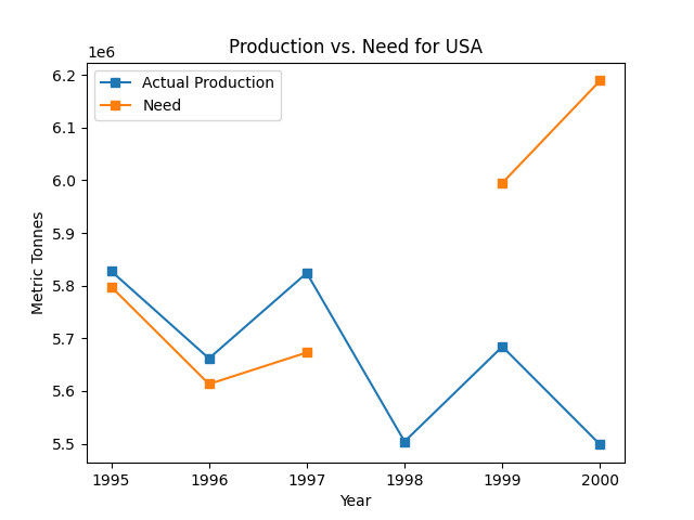
For this problem, you will create a plot of a country’s estimated production excess or deficit over time. If a country is eating more than it produces, then it’s likely importing seafood from other countries. We can visually inspect the graph to see if and when that happened.

For example, using the US data in small.csv, we should expect to see a plot similar to the following:

Problem 3a: Plot some data¶

Write a function called plot_production_vs_consumption(data, country_code) that will accept a dictionary of data returned from Problem 1’s parse_data as the first parameter and a country code as the second parameter. It will then create a plot of the country’s actual production vs. necessary production over time. You will use the functions written in problems 2a and 2b to get the data values needed for this plot.

A general approach to this problem would follow these steps:

2. Using the values from the "min_year" and "max_year" keys in the data dictionary from Problem 1, generate a list of all years between the two (inclusive). For example, with min of 1950 and max of 1955, you’d generate [1950, 1951, 1952, 1953, 1954, 1955].
3. Build up two lists, one for “actual” production, and one for production necessity:
   • For each year, use the get_actual_production function to get the production value for the country and the year and add it to the “actual” production list.
   • For each year, use the get_production_need function to get the production need value for the country and the year and add it to the “need” production list.
4. Plot the two lists of data on a line graph. You will need two calls to plt.plot() to do this, each call will use the years list for the x parameter.
   • Because there may be missing data in the “y” values, you should also add the marker='s' parameter to the plt.plot() calls.

Additionally, the plot should have the following attributes:

• xlabel is set to "Year"
• ylabel is set to "Metric Tonnes"
• title is set to "Production vs. Need for {country_code}"
• The legend is added, using plt.legend()
• Nothing else should be added to this plot; following these instructions should result in a nearly-identical plot as shown above. (Minor differences between operating systems may occur.)

You should then use plt.savefig("us-prod-vs-need.png") to save the plot as a PNG image.

Problem 3b: Pause and Interpret the Graph¶

Pause for a few minutes to think about the plot created in Problem 3a and think about the following questions.

1. When did the US’s need surpass its production?
2. What’s missing from the data we gave you that would help explain why the US was still able to consume more seafood than it produced?

Write your answers to this questions in answers.txt

Problem 4: Seeing the future¶

For this problem, you will create another graph showing predicted consumption. To do this, we will calculate a best-fit line using the consumption data returned from get_production_need() and extrapolate it into the future.

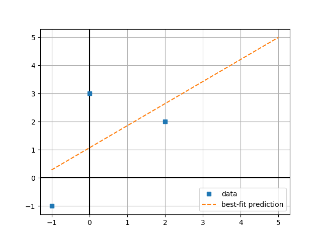
Background on best-fit lines¶

Suppose we had three 2-dimensional points, (-1, -1), (0, 3), and (2, 2). We want to find a line that best fits these points. You can visualize this as finding a line that minimizes the sum of the distances between the points and the line. As you hopefully recall from algebra, the equation for a line is typically represented as y = mx + b, where m is the slope and b is the y-intercept.

Instead of having you calculate a best-fit line by hand, we’ll use a library to calculate it for us. numpy is a huge collection of functions and tools for doing a wide range of mathematical operations, including linear algebra. One of the functions, polyfit takes in a list of x values and a list of y values and returns values we can use a m and b. With the example points above, we’d get those values with the following code:

from numpy.polynomial import polynomial as poly
xs = [-1, 0, 2]
ys = [-1, 3, 2]
b, m = poly.polyfit(xs, ys, 1)

A few things to note here:

• We import the polynomial module from the numpy.polynomial package and assign it to the name poly. This allows us to use a short version of the package name, poly.
• Even though you might often be used to seeing a list of coordinates as x, y pairs (as shown a few paragraphs earlier), numpy expects those to be separated as a list of x values and a list of y values. (Conveniently, this is also what matplotlib expects.)
• The polyfit function takes three parameters. The first two are the x and y values, respectively. The third parameter is how many polynomial terms we want. In this assignment, we’re keeping things relatively simple and only using a linear fit, so we’ll set it to 1.
• The return values for polyfit are b and then m. This is not a typo. Polyfit has far more capabilities than what we’re using it for in this assignment, and a side effect is that numpy flips things around and sees the equation as y = b + mx – the equation’s the same, but b comes before m.

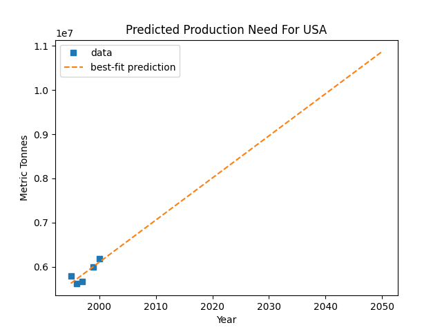
Once we have the coefficients m and b for the best-fit line, we can use the equation y = mx + b to calculate the predicted consumption for any year. In doing so, we should get a plot that looks like the following:

To make this plot line, we need to pass discrete values to matplotlib (we unfortunately can’t just give it m and b and get a line out of it). We’ll do this in two steps:

1. First, calculate a line for the best-fit line based on the results from numpy’s polyfit.
2. Second, add to that line the predicted values.

Using our list of x values, we can calculate the appropriate y on the best-fit line. In rough pseudocode, this looks like:

prediction_ys is a new list
for each x in xs:
    y = m * x + b
    add y to prediction_ys

Then, we calculate the predictions in a similar manner. We first need to generate the x values that we want prediction for, and then we can use the same equation we used for the best-fit line to calculate the y values for each prediction.

# remember range is exclusive of the last number, so we need to add one to it.
prediction_xs = list( range(max(xs) + 1, max(xs) + 4) )
for each x in prediction_xs:
    y = m * x + b
    add y to prediction_ys

And then finally, we can plot the line with the predictions using matplotlib:

plt.plot(xs + prediction_xs, prediction_ys, label='best fit prediction')

Problem 4a: Calculating best-fit prediction for US Consumption¶

Now, we’ll use the same code we used in Problem 2b (the get_production_need function) to plot the best-fit line for US consumption and a prediction out to 50 years from now.

Write a function called predict_need(data, country_code, predict_years) that returns a best-fit prediction line of production necessity data for the given country. It should return it as a dictionary in the form:

{
    "years": [...],
    "values": [...]
}

You should use the approach described in the Background on best-fit lines section above. Specifically, your code should:

1. Similar to Problem 3a, use Problem 2b‘s get_production_need function to get the observed data for each year:
   • From data["min_year"] to data["max_year"] (inclusive), append the year to a “years” list and the value from get_production_need to a “values” list.
   • Important: polyfit does not accept None values, and so if there are any None values in the data, you need to omit both the value and the year that it’s for. (The example return data below shows that even though Ankh-Morpork has some data for 1960, that year is not included in the returned data.)
2. Use poly.polyfit to calculate the best-fit line for the data. Remember:
   • Your file should have import numpy.polynomial as poly at the top. (It should already be there for you.)
   • The polyfit function takes three parameters. The first two are the x (years) and y (production need for each year) values, respectively. The third parameter should be 1.
   • polyfit returns two values, in order: b and then m.
3. Generate the values for the best-fit line and prediction.
   • Hint: You can do this in a single loop by creating a new list for both the x and y values, looping from the min year (years[0] if it’s ordered, which it should be) to the max year (years[-1]) + 51. The body of the loop would append the year to the x list, and mx + b to the y list.
4. Returns a dictionary: {"years": [...], "values": [...]}

For example, from Problem 2b above, the get_production_need function would have returned {"AMP": {1961: 10380.7687}}. In this problem, calling

predict_need(data, "AMP", 5)

would return

# (precision truncated for the spec; your actual precision will vary)
{'years': [1961, 1962, 1963, 1964, 1965, 1966], 'values': [10380.76, 10383.41, 10386.06, 10388.70, 10391.35, 10394.00]}

Problem 4b: Plotting the Prediction line¶

Now, we’ll use the predict_need function to plot the best-fit line for US consumption and a prediction out to 50 years from now.

For this problem (Problem 4b), add a line of code to call plot_linear_prediction(data, "USA") in your main code near the bottom of fishing.py (it must come after the call to parse_data). Running your program should then result in no errors and a new file named USA_need_prediction.png being created in the same folder as your program.

The plot_linear_prediction(data, country_code) function is given to you in the starter files. This function takes the output of parse_data("small.csv") as its first parameter and a country code (e.g., “USA”) as its second parameter. It then calls the predict_need function you wrote in Problem 4a with the production need data for the given country code, and then plots the best-fit line and prediction. You do not need to write this function; it’s already been written for you. But it does rely on correct implementations for previous problems.

This function has no return value, but calling plot_linear_prediction(data, "USA") should produce a plot that resembles the following:

Problem 5: Total World-wide Production Need¶

Problem 5a:¶

So, now that we’ve done all that work, how much seafood will the entire world need to produce 50 years from now?

For this problem, write a function called total_production_need(data, years_to_predict) that returns a single number: how many metric tonnes will the world need to produce years_to_predict years from now?

This function should do the following:

1. Take as input the data returned from Problem 1’s parse_data and a number of years in the future to predict.
2. For each country code, predict the production need for years_to_predict years from now using Problem 4a’s predict_need function.
3. Get the last value in the predicted values.
   • For example, if you assign the return value from predict_need to prediction, you should be able to get the last value with prediction["values"][-1].
4. Sum up all of the predicted values.
5. Return the total.

Running your program with small.csv as the input file to parse_data, total_production_need should return a total production need of 13243690.762868665. (Your degree of precision may vary.)

Problem 5b: Running with the large file:¶

At this point, it’s time to run with the larger data file. Change the call to parse_data to use "large.csv" as its input. Then, at the very end of your program, add a print statement to print out the total you return from total_production_need. Your program should print the following:

Metric tonnes of seafood needed to be produced in 50 years: 245,636,012.094

Submit your work¶

Submit fishing.py, fishing_tests.py, and answers.txt to Gradescope.

References¶

The original data for this assignment was downloaded from Kaggle:

https://www.kaggle.com/datasets/sergegeukjian/fish-and-overfishing

(That Kaggle entry is itself a repost of data from the “rfordatascience” project, which has much easier to read descriptions of the data.)

The *actual* provenance of the data comes from a variety of sources collated on ourworldindata.org:

https://ourworldindata.org/fish-and-overfishing

Each of the charts on that site have links to detailed descriptions of the data as well as references to original sources and raw data downloads.

It has a lot more data than what we’ve included in this assignment, some of which might be interesting. For example:

• https://ourworldindata.org/grapher/regulation-illegal-fishing
• https://ourworldindata.org/grapher/wild-fish-allocation
• https://ourworldindata.org/grapher/fish-landings-and-discards
• https://ourworldindata.org/grapher/bottom-trawling

Others are more summary-oriented and may be useful as additional “background” for the assignment. For example:

• https://ourworldindata.org/grapher/fish-stocks-within-sustainable-levels
• https://ourworldindata.org/grapher/global-aquaculture-wild-fish-feed
• https://ourworldindata.org/grapher/employed-fisheries-aquaculture-time

The “best-fit” calculation is done using a method called “Least Squares”. The result of that calculation is then used in Polynomial Regression. Setting polyfit‘s “deg” parameter (the third in our usage here) to 1 effectively makes it do a Linear Regression.

These are rather advanced topics, and so we do not expect you to read further into these. But the reading is provided here should you be interested or at least want to know the formal terms for what we’ve done here.