
Turn in both hardcopy in class and files by the turnin program on November 29 as specified below. Although you have 2 weeks to complete this assignment, I urge you to get as much done as possible the first week, since additional problems will be assigned during the second week.
Bender the Robot is staggering around a building in a seemingly random manner. In each room there is a motion sensor. Unfortunately, the motion sensors are quite inaccurate: there is a high probability of both a sensor failing to detect Bender when he is in the room (false negative), and firing when Bender is not in the room (false positive).
You task is to write a particle filter that tracks Bender's progress through the building. Your program takes as input a data set, and produces as output a representation of the tracker's belief state at each moment in time. We will provide several data sets to test your algorithm, as well as a copy of the simulator we use to generate the data. You may work on this alone or in teams of two people. You may use any programming language.
The world is represented by an XMAX by YMAX grid. Each cell is either a
wall or an open space (that might be occupied by the robot). There is a sensor in every non-wall square, that fires (value 1)
if it senses the robot, where the sensor error probabilities are SENSOR_FALSE_POS and
SENSOR_FALSE_NEG. After each step, the robot decides whether or not to
move with probability
MOTION_PROB. If it decides to move, then it moves with equal probability
to any adjacent open square. This continues for TMAX steps.
Data files are of the form:
XMAX YMAX
SENSOR_FALSE_POS SENSOR_FALSE_NEG MOTION_PROB
TIME_STEP SENSOR_X_COORD SENSOR_Y_COORD
SENSOR_READING
TIME_STEP SENSOR_X_COORD SENSOR_Y_COORD
SENSOR_READING
etc.
Coordinates are base 0, so the upper left-hand square is (0,0). The SENSOR_READING is 1 (fires) or 0 (does not fire) and is given for every sensor for every time slice.
The first observation is made at time 1 (not time 0).
This is a change from the original assignment
specification!
Here is an example of the first part of a data file:
5 5
0 1 0 0 0
0 0 0 1 0
1 0 1 1 0
1 0 0 0 0
1 0 0 0 1
0.100000 0.600000 0.300000
400
1 0 0 0
1 0 2 0
1 0 3 0
1 0 4 0
1 1 0 1
1 1 1 0
1 1 2 0
1 1 4 0
1 2 1 0
1 2 4 1
1 3 1 0
1 3 2 0
1 3 3 0
1 3 4 0
1 4 1 0
1 4 2 0
1 4 3 0
2 0 0 1
2 0 2 0
2 0 3 0
2 0 4 0
etc.
In this example, at time 1 the sensors in room (1,0) and (2,4) fired.
Your program should take the following command-line arguments in the order specified:
Your program writes output to the belief state file and the max belief state file. The belief state file specifies for each time step and (non-wall) location the probability that the robot is at that location. It is a series of lines of the form:
TIME_STEP X_COORD Y_COORD PROBABILITY
Note that for a given time step the probabilities for all the locations must sum to one. The max belief state file specifies the most likely location at each time step. It is a series of lines of the form:
TIME_STEP X_COORD Y_COORD
If two locations have the same probability, then break ties randomly.
The data sets are in this zip file which you should download:
See the README file for file naming conventions. The zip file also contains
New! Here is a data for a single run in a really big domain - a 100 by 100 grid. Give it a try! (But don't print out your solution, just give the summary - it is 1,000 steps long!)
The basic particle filtering algorithm is:
Initialize particles S randomly with weight 1
For each observation yt {
	For each particle s in S {
		Choose a sample s’ according to P(Xt=value(s)’|Xt-1=value(s))
		s = s’
		w(s) = P(Yt=yt|Xt=value(s)) * w(s)
	}
	After every K-th observation is processed {
		Randomly select (with replacement) a new set of particles S’ according to the distribution {w(s) | s in S}
		S = S’
		For all s in S { w(s)=1 }
	}
	For each location x {
		Compute P(Xt=x | y1, …, yt) as:
			Sum( w(s) | s in S & value(s)=x ) / Sum( w(s) | s in S )
		Print t, x, P(Xt=x | y1, …, yt)
	}
}
Represent the set of particles by an array. Each particle contains a specific X,Y coordinate of the robot's location and a weight. Note that you only need to keep track of two sets of particles, the current set of particles, and a set used for resampling the particles.
The reading from each sensor is independent given the location of the robot. Therefore the probability of the readings of all the sensors at a time step given the robot's location is the product of the probability of each sensor reading given the robot's location. Suppose the locations are just (0,0), (0,1), and (1,0). Then:

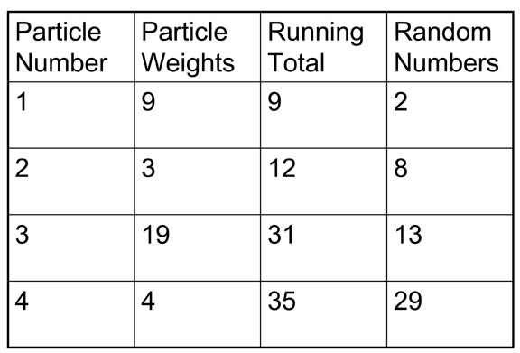
A good way to implement resampling is as follows. Convert the weights associated with each particle to integers by multiplying them by a large number and then storing the result in an array of type integer. (Note that you can just add an extra field for this purpose to the definition of a particle. Be sure to do a sanity check that the "large number" you choose isn't so large as to lead to overflow, or so small that everything gets value 0. One way to select the number is to find the heaviest weighted particle with weight w, and then multiply by (1/w)*(2<<16). Then sum up all the integer weights, call the result TOTAL. Then generate an array of size the number of particles of random numbers between 0 and TOTAL, and sort the array. Finally, simultaneously step through the random number array and the array of old particles. Each random number corresponds to a sampled particle, where the old particle is chosen so that the running sum of integer weights up to that particle is the smallest that is greater than the random number. For example, for the following arrays particle #1 is sampled twice, particle #2 is never chosen, particle #3 is sampled twice, and particle #4 is never sampled.
You will need to empirically determine settings for the number of particles and sampling frequency that give good results on the data sets. Do not expect to get 100% accuracy, that is in general not possible with noisy data.
For extra credit, also create a file that contains the most likely sequence of states the robot visits. The format of this file is the same as the max belief state file, but remember that the most likely sequence need not be same as the sequence of most likely individual states! You can compute this by augmenting each particle with a history of the location represented by that particle at each time step. At the end of the run, pick a particle that has the highest weight (breaking ties randomly) and print out its history.
This problem is small enough to solve exactly using a Hidden Markov Model. Find software for working with HMM's, figure out how to model this problem with it, and use it to calculate an exact solution to each problem. How good is the particle filtering approximation?
In class hand in printouts of your code, each max belief state file, and the percentage of the entries for each max belief state file that are the same as the corresponding entries in the ground truth files for each problem. (Do not print out the entire belief state files, only the max belief state files.)
Turn in electronic versions of these files plus the belief state files using the turnin program. If you worked in a team only hand and turn in one copy of everything.