Contents
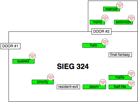
LogisticsCurrently, five of the machines in Sieg 324 are equipped
with network-enabled computers and USRP devices. They are
Each USRP board (and the associated machine) is a visitor on reserve. Unfortunately, the reservation system does not span 24 hours but rather 7am-7pm, so we'll have to find a work around for evening hours. The rule of thumb to follow is to always check if there is someone
logged into and using the machine when you log in
(run Getting startedEach group has an account on each of the equipped machines. The account names and passwords are in your e-mail inboxes. These machines do not share hard drive space. Please use your SVN repositories to share and synchronize your code, and to make sure that your code is backed up. Check your email for SVN repository access instructions, and email Ivan if anything is awry. The default shell for each group login is bash, and the local .bashrc has been slightly modified so if you prefer a different shell please translate two bottom most lines from /etc/bashrc into your shell's config file. Getting started with echo program: The first thing you should do
is download
the echo program. Unpack it and run
If you run the same command on two different machines, they will be able to communicate over the air. Type some text and push enter; you will see output that looks like this: text Tx: len(payload) = 5 c66cc66cc66cc66cacdda4e2f28c20fc00050005746578740a55555555555555Here, text is what I typed, the next line is debug output, and the
third line is the hexadecimal encoding of the actual data that was sent out
over the air. Let's break this part down into pieces:
There are four main components of this program:
The GNU Radio project has implemented a large set of examples and a large library of signal processing blocks. I have posted a zipped package of their code tree here. The two most important directories are:
Additionally, you can obtain a list of the signal processing blocks by
looking in Physical layer project detailsStart out by capturing a sample of raw USRP
output while (1) not sending any data, and (2) while constantly
sending a single bit of data (in the bpsk modulation scheme). The
usrp_rx_cfile.py -f 2.462G -d 256 outfile
This command listens at the 2.462 frequency, decimates at the rate of
256, and saves complex values as float tuples to the
file To send out a particular wave form, use the following command: usrp_siggen.py -f 2.462G -w 0
This command constantly sends a bit set to 1 (in bpsk modulation) using the 2.462 frequency. Run these commands with the -h option to find out more about the options. After you collect some wave data into a file. You probably would
like to take a peek at the data. Here are the instructions to do this
in Matlab (if you have a linux desktop configured by the CSE techstaff
then you can find the Matlab binary
here: The first thing to do in Matlab is to read in the binary file that you've collected. Download read_complex_binary.m macro file for Matlab. This file defines a single function, namely read_complex_binary(), to read such files. Make sure that this file is in the directory from which you've invoked the Matlab binary, along with the file that you're trying to read. Use the following command to read in the file as an array of complex values: M=read_complex_binary('outfile');
Once you run this command, the variable The math behind what you're seeing ...Start by downloading our example module. Note that the installation of this module involves placing files into publicly shared library directories. Make sure that you do the following before you proceed with installation: Change all references of cse561a to cse561x where x is your group. A simple grep should do this. Note that you also have to rename some of the files in the directory structure. To install this module, do the following:
tar -xzf gr-cse561a.tar.gz
All your work will take place
inside To create a new block, copy these three files to cse561a_new_block.{cc,h,i}, and change the function definitions. More comments on gnu radio blocks are available here. Phase 2 has a couple of components. First, you have to write code to handle the frequency drift. Then you have to write code to modulate and demodulate bpsk signals. After you decode the signal into bits you must be able to identify packets -- this is called framing. Lastly, you have to make sure that your new stack (including the frequency drift handling code, the bpsk modulation, and whatever transport layer you're using) is resilient to errors. Frequency drift was demonstrated in class, but you should be able to replicate the behavior and see it in Matlab (see above). It is important to realize that the frequency drift is (for our intent) is constant. From the data values, you must learn what the value of the drift is, and then you should correct for it. As a hint, consider how the angle is changing over time, and plot where it should be. The idea is to map its observed value to the correct value. BPSK stands for binary phase-shift keying. Please read this introduction to get a grasp on what's going on. The idea here is that you want to decode a wave represented in complex values into bits. The constellation diagram for BPSK in the previous link should give you a hint. Framing is typically done by including a preamble and postamble on the packet. The idea here is that a preamble composed of a particular bit pattern should tell you when a packet begins. You also need a postamble because you don't know when a packet ends (remember, at this layer you can't peek into the packet to learn how long it is because it might contain decoding errors, and because you don't know exactly which field (if any) contains the length of the packet). It is important to regard the impact of interference on your protocol stack. You should start at the bottom of the stack with the frequency drift code. To test your code without having to introduce artificial errors, simply use a lower USRP amplitude at the sender. All python files that send data have an-a AMPL
parameter. By sending at a low enough amplitude, especially between
two USRPs that are far apart or have obsticles in the line of sight
path, you will notice (in Matlab) that your wave is not as neat as
before, in particular external RF interference, ambient or otherwise
will interfere with your signal.
As a hint, to handle interference in your frequency drift correction code, you should make sure that errors only have a local impact and do not globally impact the frequency drift calculation and correction. After you certify that your frequency drift correction code is resilient to interference, start on the modulation code. The key to making your modulation code resilient to interference is to cluster potential signal values next to the most likely intended bit, and to map the signal you receive to the most probable cluster that represents the particular bit. Lastly, notice that you may still incorrectly map signal values in the previous step (if the interference is too high). In this case, you transport layer code from Phase 1 should come to the rescue. You should apply error correcting codes, and/or checksums to make sure that bad packets are identified and dropped or rejected. Routing projectThe project description for this phase is:For assignments #1 and #2, you could assume that the network consisted of a single link, and the two endpoints of the link are the only users in the system. For assignment #3, we remove those assumptions. First, design and implement a simple but robust routing algorithm for a multihop network that delivers a packet whenever a working path exists in the network for a sufficiently long period of time. Second, design and implement a simple but robust congestion control system that achieves the full bandwidth of the network and avoids starvation for any user, for a variable number of users sharing the multihop network. Demonstrate that your solution works.Lets brake this description into three pieces: 1) Design and implement a simple but robust routing algorithm for a multihop network that delivers a packet whenever a working path exists in the network for a sufficiently long period of time 2) Design and implement a simple but robust congestion control system that achieves the full bandwidth of the network and avoids starvation for any user, for a variable number of users sharing the multihop network 3) Demonstrate that your solution works Note that step (3) applies to both (1) and (2). Therefore a better ordering might be (1) (3) (2) (3). Lets look at (1) (3) and at (2) (3) in more detail. Note that the emphasis of this part is on simple and robust. Your routing algorithm must be minimal in complexity so that you can effectively evaluate its pieces. Your routing algorithm must also be robust, by which we mean that it must gracefully handle network topology changes (arising from nodes unpredictably leaving or joining the network). Wireless networks tend to be highly dynamic; therefore robustness is an important feature for a live system.This part of the project looks devilishly complex. The next section describes a possible step-by-step approach one can take to design and implement the routing layer. An important rule of thumb to follow in creating your own steps for this project is to restrict the scope of each step to something simple and technically feasible. Naming. The notion of naming is critical to routing. Depending on the routing algorithm, different naming schemes may be considered. For example, to construct a hierarchical network topology, a node's name may encode its position in the tree (e.g. its depth, or distance from the root node). To support multicast, a simple naming scheme would relax name uniqueness - two nodes with the same name in this scheme can be considered to be in the same multicast group - a packet destined for a name will be forwarded to every node with the name. Nodes might also have multiple names (e.g. to participate in two distinct 'networks'). For your project, you should outfit your transport protocol with a minimum of two fields: a field to name the sender of the packet, and a field to name the recipient of the packet (note that TCP also uses source and destination ports to uniquely identify a flow between two nodes). Depending on your routing algorithm, you might want the packet to also include the path that the packet should use. This path can be expressed as a list of node names. Forwarding packets. Routing is a form of intelligent forwarding. In this step, implement a simple forwarding mechanism that broadcasts each packet the node receives. Once this works, make sure that packets eventually leave the network (e.g. their retransmission ends). You can do this by including a TTL field (time to live) in the packet header. Nodes that retransmit a packet decrement the TTL. Packets with TTL 0 are not retransmitted. You can also achieve the same effect with timestamps - system clocks of nodes in the lab should be synchronized fairly well. In this step, you might also want to implement queueing. Queueing is necessary to handle a backlog of packets, to smooth out the performance of a link (from the perspective of a single flow), and it is also a means of instrumenting fairness into the network. You will need queues at intermediate nodes to implement congestion control in the second part of the phase. Note that your queue design will for one determine how flows impact one another (if at all), and will determine make certain congestion control schemes easier than others. For example you may decide to use a single queue for all packets, or one queue per source-destination pair, or a queue for each node in the neighborhood (a queue for each successive hop), etc. Routing with hardcoded route tables. Before being able to discover routes, make sure that you can implement basic routing logic with static routing tables. If you use flooding, make sure that flooding is constrained (e.g. with the TTL mechanism described above). Flooding has the advantage that nodes do not need to know the global network topology - the packet is forwarded until it hits the target.If you use source routing (the source specifies the route to use for the packet), then nodes need to be able to select a route for the packet through the entire network - this requires global knowledge at each of the nodes. However, unlike flooding, source routing efficiently uses the medium. With these two schemes above you have two options - to use a single table that encodes the routes for the entire network, or use a table at each node that reflects the node's local knowledge of the network. There are route maintenance and efficiency trade-offs between the two approaches. Route discovery and repair. To be robust, the routing logic needs to survive nodes leaving the network. It must also discover new routes. Depending on your routing algorithm from the previous step, you might decide to handle these scenarios differently. For example, for flooding the route maintenance is minimal - new nodes that come into the network begin to re-broadcasting any packets they hear without needing to bootstrap into the network or alert other nodes of their presence. Likewise, when a node goes offline, the routes they provided are implicitly missing. If you use a more explicit routing scheme, nodes will have to discover new nodes. However if the new nodes do not initiate any connections nor speak unless spoken to, discovering them necessitates a signaling mechanism. New nodes must advertise themselves, perhaps with a heart-beat like mechanism. A similar mechanism (perhaps coupled with timeouts) is also necessary to discover that a node left the network. Selecting the 'best' route. Some routes are better than others - you might be optimizing for latency, congestion (see next section), minimum number of hops, etc. Flooding does not allow nodes to select paths, and unnecessarily overloads the network. To select a good route, you might want to consider the loss rate on each of the links in a route, the load or the number of concurrent flows, the availability of nodes along the route (how reliable are the intermediate nodes?). Whichever metric you decide to use, please tell us. Your design should in part be motivated by the metric of your choice. Implement and Evaluate. If you're doing stepwise refinement, your implementation will mimic some of the above transitions. Make sure to finish a single step, including the evaluation of the step before moving on. It is very useful to have evaluation results for the initial routing designs with which you merely experiment before moving on. (Hopefully) these intermediary evaluations will guide your design towards something that works. Moreover these evaluations help us understand what worked and what did not work in the designs that you've tried on your way to the final product. Think hard about your evaluations. What factors should you take into account? Do you disseminate routing information (such as routing tables, or neighbor lists) reliably? If not, then BER might be an important influence on your mechanism. If you employ a flooding algorithm, how do you decide on the right TTL value? How resilient is your routing algorithm - can it withstand node churn (nodes leaving and entering the network)? Try an experiment with a node that goes on the network and leaves every 2-3 seconds. How does this node behavior impact your ability to route efficiently? Try the same experiment with two or three nodes. How fast are routes discovered, and can you algorithm take advantage of multiple routes (by striping its flows across routes)? Different algorithms will require different evaluations. A good starting point is to list the claims that you want to make about your design, and then consider experiments that will help you prove your claims at least for some small number of topologies and node behaviors. In IP networks, congestion is typically due to overflow of queues in the network or congestion at the end-hosts (correction to the latter is also termed flow control). I recommend that you only embark on this step after you have completed the routing step above. However, you might want to design both steps to support and be aware of one another. Consider the following powerful example: upon detecting congestion on a link, the routing algorithm can try to redirect flows via other links in the network to avoid the congested link. There are different indicators of congestion. The most basic one is loss (e.g. as you've learned, TCP responds to loss by abruptly changing its window size and thereby sending rate). Another useful indicator is delay. As packets queue up in the network, the one way delay (from sender to receiver) increases. Detecting this delay accurately is difficult with USRPs, so I suggest that you stay away from this indicator. Indicators may also be explicit. An explicit indicator is usually generated by the network (in your case routing nodes) that signal to the sender that they are exceeding queue capacity or are being unfair to other flows in the system - think of these as ICMP messages in IP networks. Of course these signals may be mixed - a router might signal explicitly to the sender by dropping one of the packets (selecting which packet to drop is an interesting problem!) when the queue fills up. For this part of the phase you have to decide which congestion indicator you will use, and how you will use it to reduce the sending rate adaptively, i.e. when the network has spare capacity, you should take advantage of it and when the network is over-utilized, you should take action to return its utilization back to normal. Choose a congestion indicator. Read the above discussion, and decide on either a loss or an explicit indicator of congestion (or both!). Explicit loss indicators are fun because they are mini-protocols so they allow for better introspection. On the other hand, your transport layer recovers from losses anyway, so it isn't much more difficult to respond to loss by shrinking your sending window or decreasing the sending rate. Implement and evaluate. Implementation of the loss-based indicator should not be difficult. This information should already be carried via acknowledgements. Signaling explicit congestion is more tricky because the congestion link might be deep in the network. Packets signaling congestion then have to be routed back to the source! A few interesting questions arise - should these packets be congested controlled or do they get an infinite queue of their own at each intermediary? Perhaps the routers can use this information to decide on how to route packets (e.g. routing around the congested link), etc. Evaluating congestion control mechanisms is challenging. In these experiments you need to evaluate how fast the networks detects congestion, how fast the sender responds to congestion events, how flows interact when they are flowing through a common bottleneck, and how adaptive is your mechanism - can it detect spare capacity and take advantage of this capacity (e.g. when flows leave the network). Start out with a three hop topology with a bottleneck at the second hop. This is a simple single flow test case. Then branch out to include another sender and receiver. You might need to multiplex senders and receivers on a single USRP, perhaps by using an abstraction not unlike TCP port numbers. Please, make sure you have everything else completed before embarking on tackling fairness. Its okay if you never get to this point. Decide on what fair means. Congestion control mechanisms typically exhibit fairness. This usually means that competing flows are granted a fair share of the capacity in the network. Of course fairness is subjective, and granting an equal amount of capacity to each flow is at time nonsensical (e.g. consider two competing streams - a VoIP and a BitTorrent stream). For wireless networks, fairness is made even more problematic as different nodes have different connectivity characteristics - should a node on a lossy link receive more throughput as compensation for its poor connectivity? For your project, it suffices to provide fairness at the queue level in the intermediaries (e.g. penalize queues that are overly long). However, note that you are in essence defining a particular flavor of fairness. There is lots of room to roam in this space, feel free to define fairness as you see fit. Whichever flavor you choose, you will have to carry out evaluations to show to us that your congestion control mechanisms are indeed providing the type of fairness that you claim they provide. Have fun! Work early, work often! I'll be checking email regularly for questions, and feel free to hunt me down (in CSE 391) if you have questions. Last updated Tue Nov 20 00:36:55 PST 2007 |