 |
Project 2: Ray Tracing
|
Quick Links
- Sample Solution
- Sample Scenes
- Skeleton
- Project Roadmap
- Triangle Intersection Handout
- .ray File Format
- How to use the Debugging Display
- Tool Kit Resources(FLTK, OpenGL)
- Help Session Powerpoint Presentation
- Comparison Tool
Project Description
You will build a program calledRay that will
generate ray-traced images of complex scenes. The ray tracer
should trace rays recursively using the Whitted illumination
model.
Getting Started
To get started, checkout the skeleton code from your SVN repository. In the "scenes" subdirectory of your project folder, you'll find some sample scene files (all the files with the .ray extension). These are text files that describe some geometry and the material that should be applied to them. Refer to this page for a brief explanation.
The Trace project is a very large collection of files and object-oriented C++ code. Fortunately, you only need to work directly with a subset of it. However, you will probably want to spend a bit of time getting familiar with the layout and class hierarchy at first, so that when you code you know what classes and methods are available for your use.
The skeleton code can run in both text mode and graphics mode. Text mode is usually faster. Running without any arguments will execute the program in the graphics mode. For usage see 'ray --help'.
The starting point for where ray tracing begins, and where you will be needing to add a lot of functionality, is in the RayTracer.cpp file. This is a good file to start studying and exploring what methods get called and what they do. In addition, the raytracer features a debugging window that allows you to see individual rays bouncing around the scene. This window provides a lot of visual feedback that can be enormously useful when debugging your application. Look at this web page for a detailed explanation of how to use the debugging window.
Running the Sample
Before you begin coding, you should run the sample solution; it is linked to above. It has all of the requirements implemented, along with some extra features.
Creating Your Own Scenes
As you get into the project, you'll probably want to use some scenes of your own invention. There is a help page available about the file format. This file also describes the specifications of all the primitives you are required to implement. To create realistic refractive objects, you'll need their Indices of Refraction.
Testing Your Project
Once you implement the requirements listed below, you'll be able to test it with this automated tool. This tool compares your program's output against the sample solution's. A readme is included to help you use the tool. It is in your best interest to test with the tool, as the TAs will be using it to get a sense of how your program compares to the sample solution. Don't worry if your solution doesn't give exactly the same output (rounding errors, among other things, are a fact of life). This tool is only to get an idea of where to look for problems. Note that your bells and whistles must be disabled for the tool to accurately check against the sample.
Required Functionality
We'll describe these requirements in more detail afterwards:- The skeleton code has no triangle-ray intersection implementation. Fill in the triangle intersection code so that your ray tracer can display triangle meshes.
- The skeleton code has no sphere-ray intersection implementation. Fill in the sphere intersection code so that your ray tracer can display spheres.
- Implement the Whitted illumination model, which includes Phong shading (emissive, ambient, diffuse, and specular terms) as well as reflection and refraction terms. You only need to handle directional and point light sources, i.e. no area lights, but you should be able to handle multiple lights.
- Implement Phong interpolation of normals on triangle meshes.
- Implement anti-aliasing. Regular super-sampling is acceptable, more advanced anti-aliasing will be considered as an extension.
- Implement data structures that speed up the intersection computations in large scenes. There will be a contest at the end of the project to determine the team with the fastest ray tracer.
Notes on Whitted's illumination model
The first three terms in Whitted's model will require you to trace rays towards each light, and the last two will require you to recursively trace reflected and refracted rays. (Notice that the number of reflected and refracted rays that will be calculated is limited by the "depth" setting in the ray tracer. This means that to see reflections and refraction, you must set the depth to be greater than zero!)When tracing rays toward lights, you should look for intersections with objects, thereby rendering shadows. If you intersect a semi-transparent object, you should attenuate the light, thereby rendering partial (color-filtered) shadows, but you may ignore refraction of the light source.
The skeleton code doesn't implement Phong interpolation of normals. You need to add code for this (only for meshes with per-vertex normals.)
Here is a document that lists equations that will come in handy when writing your shading and ray tracing algorithms.
Anti-aliasing
Once you've implemented the shading model and can generate images, you will notice that the images you generated are filled with "jaggies". You should implement an anti-aliasing technique to smooth these rough edges. In particular, you are required to perform super-sampling and averaging down. You should provide a slider which allows the user to control the number of samples per pixel (1, 4, 9 or 16 samples). You need only implement a box filter for the averaging down step. More sophisticated anti-aliasing methods are left as bells and whistles below.Acclerated ray-surface intersection
The goal of this portion of the assignment is to speed up the ray-surface intersection module in your ray tracer. In particular, we want you to improve the running time of the program when ray tracing complex scenes containing large numbers of objects (they are usually triangles). There are two basic approaches to do this:- Specialize and optimize the ray-object intersection test to run as fast as possible.
- Add data structures that speed the intersection query when there are many objects.
Most of your effort should be spent on approach 2, i.e. reducing the number of ray-object intersection tests. You are free to experiment with any of the acceleration schemes described in Chapter 6, ''A Survey of Ray Tracing Acceleration Techniques,'' of Glassner's book. Of course, you are also free to invent new acceleration methods.
Make sure that you design your acceleration module so that it is able to handle the current set of geometric primitives - that is, triangles spheres, squares, boxes, and cones.
The sample scenes include several simple scenes and three complex test scenes: trimesh1, trimesh2, and trimesh3. You will notice that trimesh1 has per-vertex normals and materials, and trimesh2 has per-vertex materials but not normals. Per-vertex normals and materials imply interpolation of these quantities at the current ray-triangle intersection point (using barycentric coordinates).
Acceleration grading criteria
The test scenes each contain up to thousands of triangles. A portion of your grade for this assignment will be based on the speed of your ray tracer running on these scenes. The faster you can render a picture, the higher your grade.
For grading on the rendering speed, the scenes will be traced at the specific size with one ray traced per pixel, and the rays should be traced with 5 levels of recursion, i.e. each ray should bounce 5 times. If during these bounces you strike surfaces with a zero specular reflectance and zero refraction, stop there. At each bounce, rays should be traced to all light sources, including shadow testing. The command for testing rendering speed looks like:
ray -b -w 400 -r 5 in.ray out.bmp[For fairness, don't include other stop criteria (except for the one mentioned above) for -b option.]
You are welcome to precompute scene-specific (but not viewpoint-specific) acceleration data structures and make other time-memory tradeoffs, but your precomputation time and memory use should be reasonable. Don't try to customize your ray tracer for the test scenes; we will also use other scenes during grading. If you have any questions about what constitutes a fair acceleration technique, ask us. Coding your inner loops in machine language is unfair. Using multiple processors is unfair. Compiling with optimization enabled is fair. In general, don't go overboard tuning aspects of your system that aren't related to tracing rays.
Artifact Requirements
Each team is required to submit one artifact per person. Name the file <your-cse-netid>.jpg or <your-cse-netid>.png. The scene traced cannot be one of the provided .ray files but must at least be modified in some way (or a completely new scene). With each artifact, a text file describing the scene may also be submitted (<your-cse-netid>.txt). This can be as simple as two sentences describing the placement of the objects and lights to get the desired effect or a detailed description of the bells and whistles used to create the scene. The text file will be linked with your artifact.
If you implement any bells or whistles you need to provide examples of these features in effect. You should present your extra credit features at grading time either by rendering scenes that demonstrate the features during the grading session or by showing images you rendered in advance. You might need to pre-render images if they take a while to compute (longer than 30 seconds). These pre-rendered examples, if needed, must be included in your turnin directory on the project due date. The scenes you use for demonstrating features can be different from what you end up submitting as an artifact.
Bells and Whistles
This assignment is large, and, furthermore, the optimization element is completely open-ended, so you can profitably work on that until the project is due. Therefore we don't neccessarily expect a bunch of bells and whistles. We can't stop you, though. Below are some interesting extensions to this project.
Both Shirley's book and Foley, et al., are reasonable resources for implementing bells and whistles. In addition, Glassner's book on ray tracing is a very comprehensive exposition of a whole bunch of ways ray tracing can be expanded or optimized (and it's really well written). If you're planning on implementing any of these bells and whistles, you are encouraged to read the relevant sections in these books as well.
Remember that you'll need to establish to our satisfaction that you've implemented the extension! You should have test cases that clearly demonstrate the effect of the code you've added to the ray tracer. Sometimes different extensions can interact, making it hard to tell how each contributed to the final image, so it's also helpful to add controls to selectively enable and disable your extensions. In fact, we require that all extensions be disabled by default, with controls to turn them on one by one.
Here are some examples of effects you can get with ray tracing. Currently none of these were created from past students' ray tracers.
![]()
Implement stochastic (jittered) supersampling. See Glassner, Chapter
5, Section 4.1 - 4.2 and the first 4 pages of Section 7.
![]() Modify shadow attenuation to use Beer's law, so that the thicker objects cast darker
shadows than thinner ones with the same transparency constant. (See Shirley p. 214.)
Modify shadow attenuation to use Beer's law, so that the thicker objects cast darker
shadows than thinner ones with the same transparency constant. (See Shirley p. 214.)
![]() Include a Fresnel term so that the amount of reflected and refracted light at a
transparent surface depend on the angle of incidence and index of refraction. (See Shirley p. 214.)
Include a Fresnel term so that the amount of reflected and refracted light at a
transparent surface depend on the angle of incidence and index of refraction. (See Shirley p. 214.)
![]() Add a menu option that lets you
specify a background image to replace the
environment's ambient color during the rendering. That is, any ray
that goes off into infinity behind the scene should return a color from the
loaded image, instead of just black. The background
should appear as the backplane of the rendered image with suitable
reflections and refractions to it.
Add a menu option that lets you
specify a background image to replace the
environment's ambient color during the rendering. That is, any ray
that goes off into infinity behind the scene should return a color from the
loaded image, instead of just black. The background
should appear as the backplane of the rendered image with suitable
reflections and refractions to it.
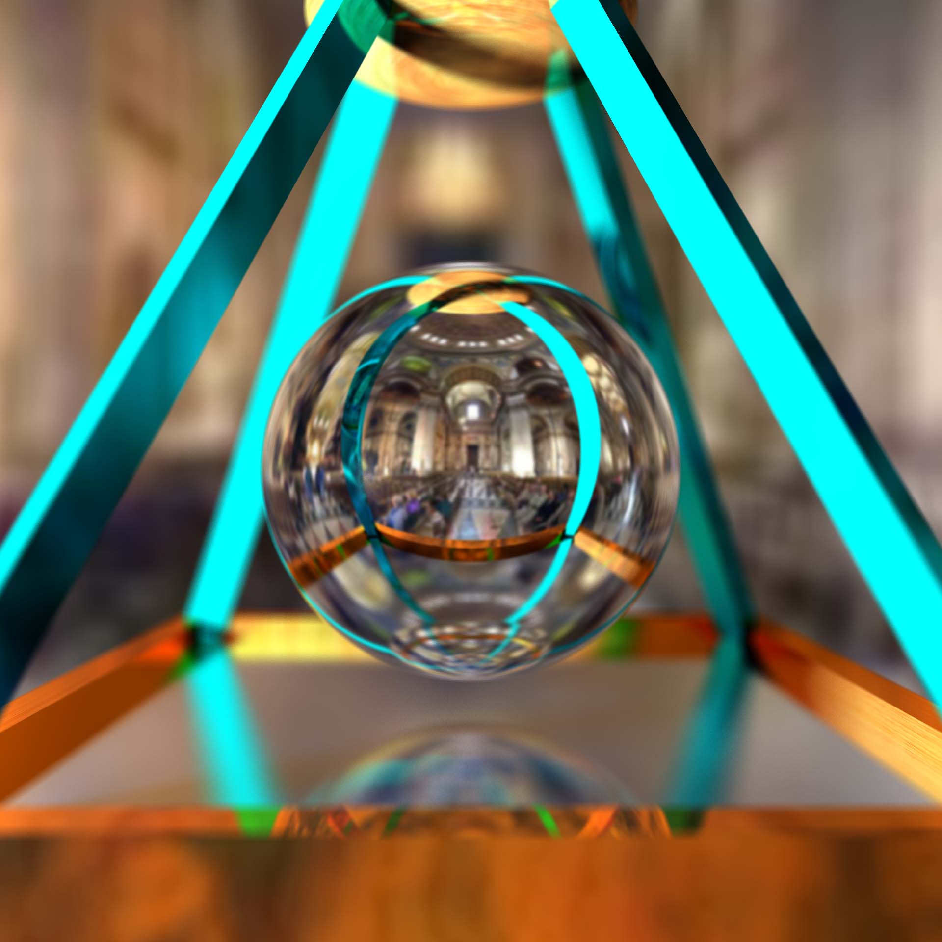
![]() Deal with overlapping objects intelligently. In class, we
discussed how to handle refraction for non-overlapping objects in air.
This approach breaks
down when objects intersect or are wholly contained inside other
objects. Add support to the refraction code for detecting this and handling it
in a more realistic fashion. Note, however, that in the real world, objects can't coexist
in the same place at the same time. You will have to make assumptions as to
how to choose the index of refraction in the overlapping space. Make
those assumptions clear when demonstrating the results.
Deal with overlapping objects intelligently. In class, we
discussed how to handle refraction for non-overlapping objects in air.
This approach breaks
down when objects intersect or are wholly contained inside other
objects. Add support to the refraction code for detecting this and handling it
in a more realistic fashion. Note, however, that in the real world, objects can't coexist
in the same place at the same time. You will have to make assumptions as to
how to choose the index of refraction in the overlapping space. Make
those assumptions clear when demonstrating the results.
![]() Implement spot lights.
Implement spot lights.
![]() Implement antialiasing
by adaptive supersampling, as described in Glassner, Chapter 1,
Section 4.5 and Figure 19 or in Foley, et al.,
15.10.4. For full credit, you must show some sort of visualization of the
sampling pattern that results. For example, you could create another
image where each pixel is given an intensity proportional to the number of
rays used to calculate the color of the corresponding pixel in the ray
traced image. Implementing this bell/whistle is a big win -- nice
antialiasing at low cost.
Implement antialiasing
by adaptive supersampling, as described in Glassner, Chapter 1,
Section 4.5 and Figure 19 or in Foley, et al.,
15.10.4. For full credit, you must show some sort of visualization of the
sampling pattern that results. For example, you could create another
image where each pixel is given an intensity proportional to the number of
rays used to calculate the color of the corresponding pixel in the ray
traced image. Implementing this bell/whistle is a big win -- nice
antialiasing at low cost.
![]() Add some new
types of geometry to the ray tracer. Consider implementing
torii or general quadrics. Many other objects are possible
here.
Add some new
types of geometry to the ray tracer. Consider implementing
torii or general quadrics. Many other objects are possible
here.
![]() Implement more versatile lighting controls, such as the Warn model described in Foley 16.1.5.
This allows you to do things like control the shape of the projected light.
Implement more versatile lighting controls, such as the Warn model described in Foley 16.1.5.
This allows you to do things like control the shape of the projected light.
![[Bell]](images/bell.gif) for the first, for each additional
for the first, for each additional
Implement stochastic or distributed ray tracing to produce one or more or the following effects: depth of field, soft shadows, motion blur, glossy reflection (See Glassner,
chapter 5, or Foley, et al., 16.12.4).
![]()
![]() Add texture mapping support to the program. To get full credit for this, you must add uv coordinate mapping
to all the built-in primitives (sphere, box, cylinder, cone) except trimeshes. The square object already has
coordinate mapping implemented for your reference. The most basic kind of texture mapping is to apply the map
to the diffuse color of a surface. But many other parameters can be mapped. Reflected color can be mapped to create
the sense of a surrounding environment. Transparency can be mapped to create holes in objects. Additional (variable)
extra credit will be given for such additional mappings. The basis for this bell is built into the skeleton, and the
parser already handles the types of mapping mentioned above. Additional credit will be awarded for quality implementation
of texture mapping on general trimeshes.
Add texture mapping support to the program. To get full credit for this, you must add uv coordinate mapping
to all the built-in primitives (sphere, box, cylinder, cone) except trimeshes. The square object already has
coordinate mapping implemented for your reference. The most basic kind of texture mapping is to apply the map
to the diffuse color of a surface. But many other parameters can be mapped. Reflected color can be mapped to create
the sense of a surrounding environment. Transparency can be mapped to create holes in objects. Additional (variable)
extra credit will be given for such additional mappings. The basis for this bell is built into the skeleton, and the
parser already handles the types of mapping mentioned above. Additional credit will be awarded for quality implementation
of texture mapping on general trimeshes.
![]()
![]() Implement bump mapping (Watt 8.4; Foley, et al. 16.3.3).
Check this out!
Implement bump mapping (Watt 8.4; Foley, et al. 16.3.3).
Check this out!
![]()
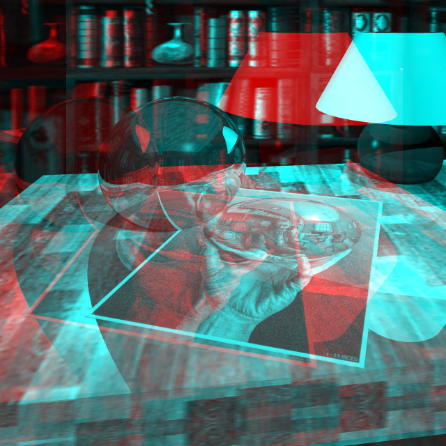
![]() Extend the ray-tracer to create Single Image Random Dot Stereograms
(SIRDS). Click here to read a paper
on
how to make them. Also check out this page of examples.
Or, create 3D images like this one, for viewing
with red-blue glasses.
Extend the ray-tracer to create Single Image Random Dot Stereograms
(SIRDS). Click here to read a paper
on
how to make them. Also check out this page of examples.
Or, create 3D images like this one, for viewing
with red-blue glasses.
![]()
![]()
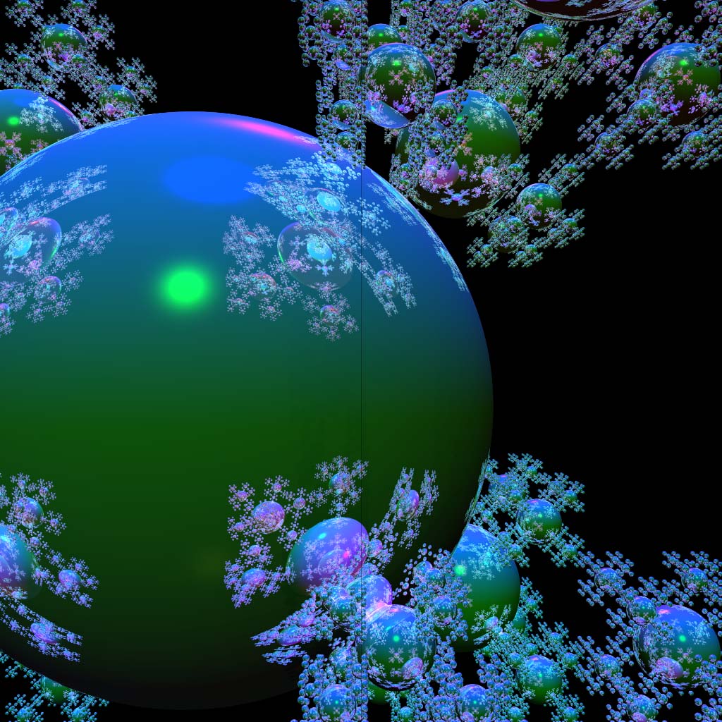
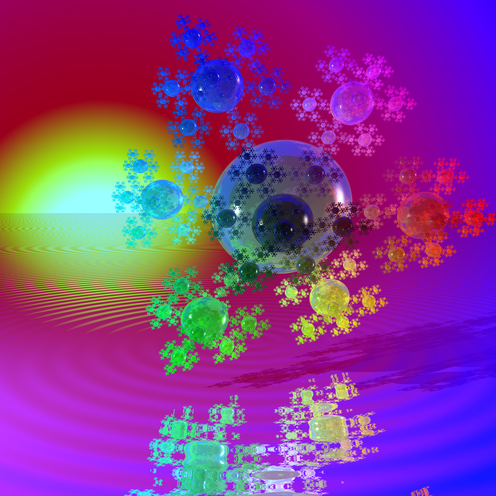
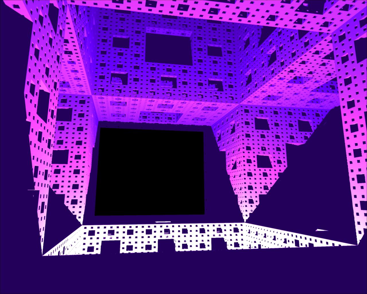
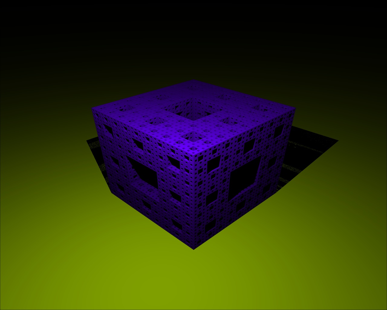
![]() Implement 3D fractals and extend the .ray file format
to provide support for these objects. Note that you are not allowed to "fake" this by
just drawing a plain old 2D fractal image, such as the usual Mandelbrot Set. Similarly, you
are not allowed to cheat by making a .ray file that arranges objects in a fractal pattern,
like the sier.ray test file. You must raytrace an actual 3D fractal, and your extension
to the .ray file format must allow you to control the resulting object in some interesting
way, such as choosing different fractal algorithms or modifying the base pattern used to produce the fractal.
Implement 3D fractals and extend the .ray file format
to provide support for these objects. Note that you are not allowed to "fake" this by
just drawing a plain old 2D fractal image, such as the usual Mandelbrot Set. Similarly, you
are not allowed to cheat by making a .ray file that arranges objects in a fractal pattern,
like the sier.ray test file. You must raytrace an actual 3D fractal, and your extension
to the .ray file format must allow you to control the resulting object in some interesting
way, such as choosing different fractal algorithms or modifying the base pattern used to produce the fractal.
Here are two really good examples of raytraced fractals that were produced by students during a previous quarter:
Example 1,
Example 2
And here are a couple more interesting fractal objects:
Example 3,
Example 4
![]()
![]()
![]()
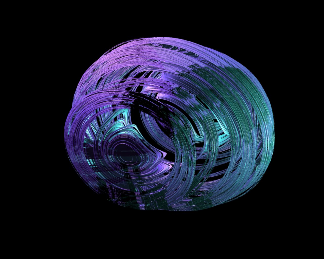
![]() Implement 4D quaternion fractals and extend the .ray file format
to provide support for these objects. These types of fractals are generated by using a generalization
of complex numbers called quaternions. What makes the fractal really interesting is that it is actually
a 4D object. This is a problem because we can only perceive three spatial dimensions, not four. In order
to render a 3D image on the computer screen, one must "slice" the 4D object with a three dimensional
hyperplane. Then the points plotted on the screen are all the points that are in the intersection of
the hyperplane and the fractal. Your extension to the .ray file format must allow you to control the
resulting object in some interesting way, such as choosing different generating equations, changing
the slicing plane, or modifying the surface attributes of the fractal.
Implement 4D quaternion fractals and extend the .ray file format
to provide support for these objects. These types of fractals are generated by using a generalization
of complex numbers called quaternions. What makes the fractal really interesting is that it is actually
a 4D object. This is a problem because we can only perceive three spatial dimensions, not four. In order
to render a 3D image on the computer screen, one must "slice" the 4D object with a three dimensional
hyperplane. Then the points plotted on the screen are all the points that are in the intersection of
the hyperplane and the fractal. Your extension to the .ray file format must allow you to control the
resulting object in some interesting way, such as choosing different generating equations, changing
the slicing plane, or modifying the surface attributes of the fractal.
Here are a few examples, which were created using the POV-Ray raytracer
(yes, POV-Ray has quaternion fractals built in!):
Example 1,
Example 2,
Example 3,
Example 4.
And, this is an excellent example from a previous quarter.
To get started, visit this web page to brush up on your
quaternion math. Then go to this site
to learn about the theory behind these fractals. Then, you can take a look at this page
for a discussion of how a raytracer can perform intersection calculations.
![]()
![]()
![]()
![]() Implement a more realistic shading model. Credit will vary depending on the sophistication of the model.
A simple model factors in the Fresnel term to compute the amount of light reflected and transmitted at a perfect
dielectric (e.g., glass). A more complex model incorporates the notion of a microfacet distribution to broaden
the specular highlight. Accounting for the color dependence in the Fresnel term permits a more metallic appearance.
Even better, include anisotropic reflections for a plane with parallel grains or a sphere with grains that follow
the lines of latitude or longitude. Sources: Shirley, Chapter 24, Watt, Chapter 7, Foley et al, Section 16.7;
Glassner, Chapter 4, Section 4; Ward's SIGGRAPH '92 paper; Schlick's Eurographics Rendering Workshop '93 paper.
Implement a more realistic shading model. Credit will vary depending on the sophistication of the model.
A simple model factors in the Fresnel term to compute the amount of light reflected and transmitted at a perfect
dielectric (e.g., glass). A more complex model incorporates the notion of a microfacet distribution to broaden
the specular highlight. Accounting for the color dependence in the Fresnel term permits a more metallic appearance.
Even better, include anisotropic reflections for a plane with parallel grains or a sphere with grains that follow
the lines of latitude or longitude. Sources: Shirley, Chapter 24, Watt, Chapter 7, Foley et al, Section 16.7;
Glassner, Chapter 4, Section 4; Ward's SIGGRAPH '92 paper; Schlick's Eurographics Rendering Workshop '93 paper.
This all sounds kind of complex, and the physics behind it is. But the coding doesn't have to be. It can be worthwhile to look up one of these alternate models, since they do a much better job at surface shading. Be sure to demo the results in a way that makes the value added clear.
Theoretically, you could also invent new shading models. For instance, you could implement a less realistic model! Could you implement a shading model that produces something that looks like cel animation? Variable extra credit will be given for these "alternate" shading models. Links to ideas: Comic Book Rendering
Note that you must still implement the Phong model.
![]()
![]()
![]()
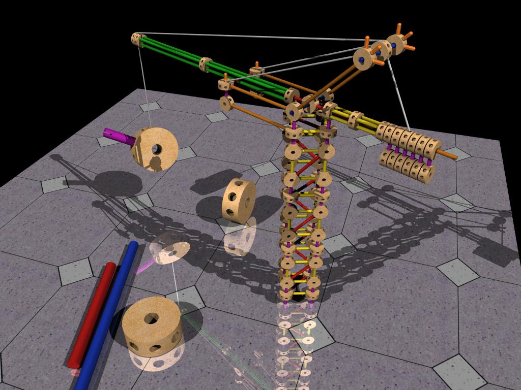
![]() Implement CSG, constructive solid geometry. This extension allows you to create very interesting models.
See page 108 of Glassner for some implementation suggestions. An excellent example of CSG
was built by a grad student here in the grad graphics course.
Implement CSG, constructive solid geometry. This extension allows you to create very interesting models.
See page 108 of Glassner for some implementation suggestions. An excellent example of CSG
was built by a grad student here in the grad graphics course.
![]()
![]()
![]()
![]() Add a particle systems simulation and renderer (Foley 20.5, Watt 17.7, or see instructor for more pointers).
Add a particle systems simulation and renderer (Foley 20.5, Watt 17.7, or see instructor for more pointers).
![]()
![]()
![]()
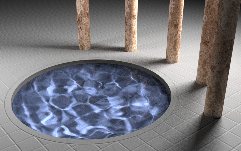
![]() Implement caustics by tracing rays from the light source and depositing energy in texture maps
(a.k.a., illumination maps, in this case). Caustics are variations in light intensity caused by refractive
focusing--everything from simple magnifying-glass points to the shifting patterns on the bottom of a swimming pool.
A paper discussing some methods. 2 bells each for refractive and reflective caustics.
(Note: caustics can be modeled without illumination maps by doing "photon mapping", a monster bell described below.)
Implement caustics by tracing rays from the light source and depositing energy in texture maps
(a.k.a., illumination maps, in this case). Caustics are variations in light intensity caused by refractive
focusing--everything from simple magnifying-glass points to the shifting patterns on the bottom of a swimming pool.
A paper discussing some methods. 2 bells each for refractive and reflective caustics.
(Note: caustics can be modeled without illumination maps by doing "photon mapping", a monster bell described below.)
Here is a really good example of caustics that were produced by two students during a previous quarter: Example
There are innumerable ways to extend a ray tracer. Think about all the visual phenomena in the real world. The look and shape of cloth. The texture of hair. The look of frost on a window. Dappled sunlight seen through the leaves of a tree. Fire. Rain. The look of things underwater. Prisms. Do you have an idea of how to simulate this phenomenon? Better yet, how can you fake it but get something that looks just as good? You are encouraged to dream up other features you'd like to add to the base ray tracer. Obviously, any such extensions will receive variable extra credit depending on merit (that is, coolness!). Feel free to discuss ideas with the course staff before (and while) proceeding!
Disclaimer: please consult the course staff before spending any serious time on these. These are all quite difficult (I would say monstrous) and may qualify as impossible to finish in the given time. But they're cool.
![]()
![]()
![]()
![]()

![]()
![]()
![]()
![]()
Sub-Surface Scattering
The trace program assigns colors to pixels by simulating a ray of light that travels, hits a surface, and then leaves the surface at the same position. This is good when it comes to modeling a material that is metallic or mirror-like, but fails for translucent materials, or materials where light is scattered beneath the surface (such as skin, milk, plants... ). Check this paper out to learn more.
![]()
![]()
![]()
![]()
![]()
![]()
![]()
![]()
Metropolis Light Transport
Not all rays are created equal. Some light rays contribute more to the image than others, depending on what they reflect off of or pass through on the route to the eye. Ideally, we'd like to trace the rays that have the largest effect on the image, and ignore the others. The problem is: how do you know which rays contribute most? Metropolis light transport solves this problem by randomly searching for "good" rays. Once those rays are found, they are mutated to produce others that are similar in the hope that they will also be good. The approach uses statistical sampling techniques to make this work. Here's some information on it, and a neat picture.
![]()
![]()
![]()
![]()
![]()
![]()
![]()
![]()
Photon Mapping
Photon mapping is a powerful variation of ray tracing that adds speed, accuracy and versatility. It's a two-pass method: in the first pass photon maps are created by emitting packets of energy photons) from the light sources and storing these as they hit surfaces within the scene. The scene is then rendered using a distribution ray tracing algorithm optimized by using the information in the photon maps. It produces some amazing pictures. Here's some information on it.
Also, if you want to implement photon mapping, we suggest you look at the SIGGRAPH 2001 course 38 notes. The TA's can point you to a copy, if you are interested.
References
- General
- An Improved Illumination Model for Shaded Display, T. Whitted, CACM, 1980, pp 343-349
- An Introduction to Ray Tracing, Andrew S. Glassner. (Chap. 6 for acceleration)
- Space Subdivision
- Ray Tracing with the BSP Tree, K Sung & P. Shirley. Graphics Gems III.
- ARTS: Accelerated Ray-Tracing System, A. Fujimoto et. al. CG&A April 1986, pp 16-25.
- A Fast Voxel Traversal Algorithm for Ray Tracing, J. Amanatides & A. Woo. Eurographics'87, pp 3-9
- Faster Ray Tracing Using Adaptive Grids, K. Klimaszewski & T. Sederberg. CG&A Jan. 1997, pp 42-51 (It is claimed to be the fastest algorithm so far.)
- Hierarchical Bounding Volume
- Automatic Creation of Object Hierarchies for Ray Tracing, J. Goldsmith & J. Salmon. CG&A May 1987, pp 14-20.
- Efficiency Issues for Ray Tracing, B. Smits. Journal of Graphics Tools, Vol. 3, No. 2, pp. 1-14, 1998.
- Ray Tracing News, Vol. 10, No. 3.
- Tips
- Fast Ray-Box Intersection, A. Wu Graphics Gems.
- Improved Ray Tagging for Voxel-Based Ray Tracing, D. Kirk & J. Arvo. Graphics Gems. II
- Rectangular Bounding Volumes for Popular Primitives, B. Trumbore. Graphics Gems. III
- A Linear-Time Simple Bounding Volumn Algorithm, X. Wu. Graphics Gems. III
- A Fast Alternative to Phong's Specular Model, Christophe Schlick Graphics Gems IV.
- Voxel Traversal along a 3D Line, D. Cohen. Graphics Gems. IV.
- Faster Refraction Formula, and Transmission Color Filtering, Ray Tracing News, Vol. 10, No. 1.