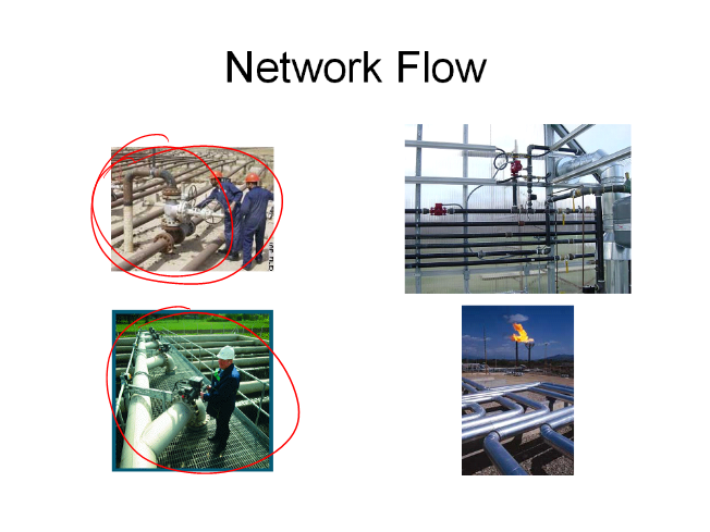
This slide has a pictorial introduction to network flow. It is important to realize that network flow is best modelled by thinking about liquid flowing through pipes - not packets through a computer network.
There is some joking around with the UW students about networks. At 1:15 a student asks "Are these accurate representations of the internet according to a senator from Alaska". This refers to comments made by Senator Ted Stevens describing the Internet as a series of tubes. This can be ignored.

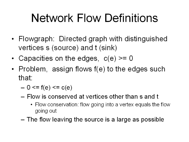
The basic definitions of network flow. At about 4:30 a student asks if there are only one source or sink. The answer is that the version we consider in this lecture has one source and one sink (but in lecture 24 we give a version of flow with multiple sources and sinks).

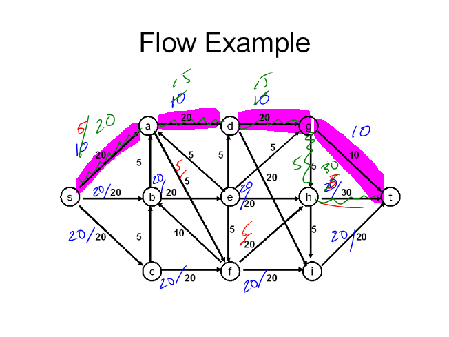
This slide gives an example of network flow. The question of what is the maximum flow is asked at 7:05. You probably want to stop here and get an answer. A number of students at UW shouted out the correct answer of 30, although that isn't audible on the tape.
At 8:05 the example shows 20 units of flow. A student points out how another 10 units of flow can be sent.

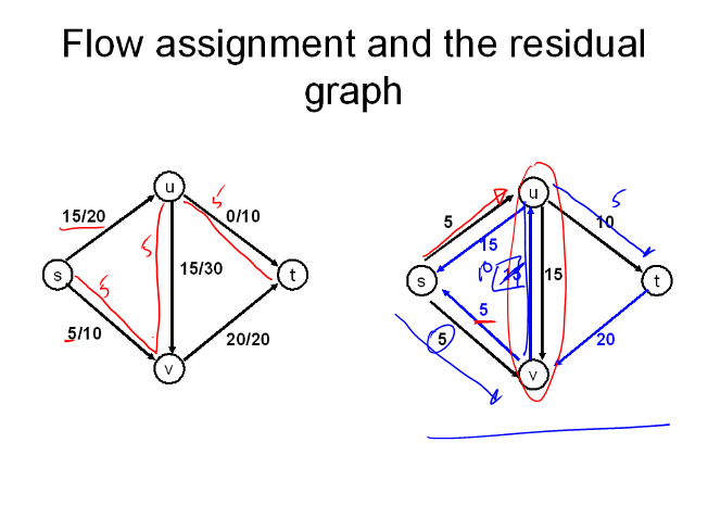
Quite a bit of time is spent on this slide since augmenting the flow by using the residual graph is the key idea of the algorithm.
The instructor works through an example. This is done interactively with the students. At 15:50 the instructor has a flow of size 50, and asks the students if he is stuck. Students point out how to increase the flow. (The student comment is unusually clear).
A similar example is given to the students to work on. Some of the edge capacities have been changed, but the edge structure is the same. Students worked on this for about 5 minutes. By the time students submitted their answers, the majority had discovered the correct solution of size 65.
The instructor looked through student solutions without comment, then at 23:55 he asked if anyone had found a flow of 70.

The instructor reconstructs the solution (this is the same network as used for the submission), and then points out that we couldn't do more than 70 units. At 26:00 he asks if we could do more than 65 units. This would be a good time to stop for a discussion.
The students provide a couple of different answers, where they identify different cuts in the graph that bounds the total flow. This relationship between cuts and flows is very important.

This is the natural midpoint of the lecture if this is to be split over two sessions.
Augmenting paths are discussed on this slide. Two types of paths are illustrated - an augmentation that adds to flow, and an augmentation which sends flow in the reverse direction. The latter type of augmentation is illustrated at about 30:35. This is the key idea from the slide.

This student submission is to reinforce the ideas from the previous slide by finding two augmenting paths. There was quite a bit of discussion between students as they determined what the answers was. I thought this was quite effective at having students explain to each other what augmenting paths were. When solutions were displayed, they were all correct.

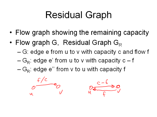
The residual graph is introduced - this is covered quite carefully, with a description, an example, and then a submission. The student submission activity is mechanical - so you shouldn't spend too much time on it.

At 41:45 the instructor asks what is the maximum flow. THe instructor points out the cut that is saturated.
The point that came up in discussion of the residual graph is that there is a bug on the slide - node g has 4 units going in, but only 3 units going out. (This may have been corrected on the ppt slide deck - but is incorrect on the webviewer version).

The final discussion gives a summary of the algorithm that we will use for network flow. This algorithm is the Ford-Fulkerson algorithm, and it is covered in detail in lecture 23.
