
There are no activity slides in this lecture. The instructor does a few activities through verbal interaction with the students, and this is probably going to be the best approach for you as well, given the difficulty of the subject matter. It would be better if you stopped the video at these spots and re-created the discussion locally. Since in this lecture you should stop pretty much every time the instructor asks a question, I haven't marked which interactions you should stop for
This lecture presents a memory-efficient algorithm for finding the LCS.

Here the instructor reviews the LCS problem.

In the original dynamic programming algorithm, the key idea was how we broke the problem into m*n subproblems.


To compute the value at a node, we must compute the value of all three of its predecessors.

This is a review of the original dynamic programming algorithm.
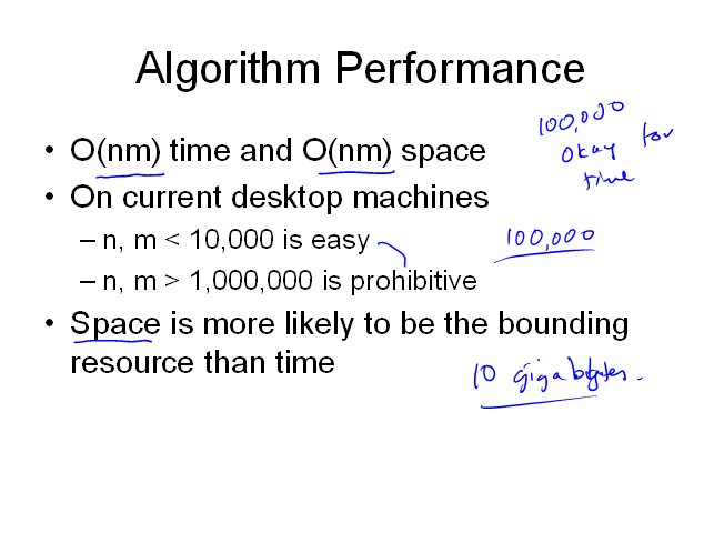
Here we review the time and space performance of the original algorithm; this is the motivation for the algorithm we see today.
At 6:30, the instructor asks, "What were out thoughts last time about feasibility?" A student responds, "It was ok for time but not for space."
At 7:14, the instructor says, "Remind me what we were getting for space?" A student responds, "Several gigabytes."
At 7:36, the instructor asks, "How many of you have 10 gigabytes on your home machine?" There is no response.

We saw that space is the constraining resource, so today's algorithm works to improve space. To start to see how this could be done, the instructor discusses how the algorithm to find the length of an LCS can be run in O(n+m) space. At 8:48, the instructor asks, "Why is that?" A student responds, "You only really need the previous row or column."
The point here is that, in the original algorithm, you only need the O(nm) space if you are going to recover the string.

The instructor says he finds it interesting that here we will recompute some values to save space.
At 11:56, he asks, "Has it ever been useful to use some extra space to save time?" A student responds by saying we did this in dynamic programming.
The point is that where before we used more space to save time, now we will use more time to save space.

Here the instructor presents the basic idea behind the algorithm. You look at the path you take through the matrix to recover the LCS and find where it crosses the middle column of the matrix. You then use this middle column as a dividing point for reducing the problem into smaller subproblems.

Here the instructor defines the Constrained LCS problem.
At 17:25, the instructor begins to do the example, asking the students at each step what to do. At 17:25, he asks, "What do I get for LCS 4,3 of these two strings?" He gets no response, so at 17:44 he asks, "What substrings am I pairing up?" And at 18:19, "And the second half?" I would suggest you start by asking what strings will be compared.
At 19:33, the instructor asks, "Without the constraint, what is the LCS of A and B?" Students give both of the correct responses, cbb and bba.
The point here is that putting in this constraint can reduce the quality of matches, and for our new algorithm we want to look at constrained LCSs divided on the first string by the middle column; now we just need to know where to divide B.

The instructor does this example, at each step asking the students for contributions. The point of this example is just to make it clear what we are computing.
At 21:39 the instructor asks, "The LCS 5,0 (A, B) - What is this?" A student responds, "TRTS."
At 22:40 the instructor asks, "The LCS 5,1 (A, B)?" A student responds, "R, TRTS"
At 22:40, the instructor says, "Let's do one more, what value should we do?" A student responds, "5, 4" At 24:10 the instructor asks, "What is that?" A student responds, "RSR" The instructor asks, "the second half?" A student responds, "RTS"

The instructor ties the example just done back to the diagram on slide 5.
At 28:20, he asks, " I claim that one of these gives us the optimal length of the string. Why?" A student responds, "You've considered all possible ways to break up B." So this tells us: the length of the LCS, and where to split B to find the LCS.


j is the index where we can split B such that computing LCS(a1...am/2, b1...bj) and LCS(am/2+1...m, bj+1...bn) gives the LCS(A, B).

The instructor says that the key to understanding the algorithm is understanding the recursion picture.
At 33:39, the instructor asks, "Is it clear what the algorithm is?" There is no response.
At 33:50, the instructor asks, "What is the space of this algorithm?" A student responds, "You need to maintain the table from a couple of slides ago(slide 13)"
The instructor makes the point that the size of the tables is O(n).
The instructor then begins discussing runtime, and says that it's surprising that the runtime of the algorithm is O(nm).
At 36:56, he asks, "How do we solve this type of recurrence?" There is no response.
At 37:30, he asks, "Any approaches to solving this recurrence?" A student responds, "If we knew the worst-case j, we could use that." The instructor says that that is an excellent point, but that isn't how we will do this recurrence.
At 39:18, he asks "Any other approaches?" There is no response. The instructor says that one approach is unrolling, but we won't use that here. The other approach is guess and verify, which is what we will use here. We will prove it by induction.
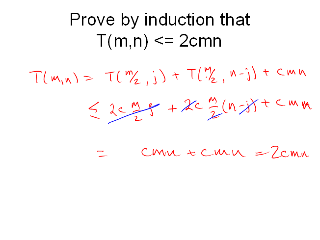
Here the instructor does the inductive proof.
At 42:18, the instructor asks, "What do we get by applying the Induction Hypothesis?" The student response is hard to hear but the instructor writes it down.
At 43:39, the instructor says that the key is that the j terms cancel out. The reason is that the amount of work we do doesn't depend upon j. That is, the amount of work is the same for every j. He then goes to the whiteboard to explain this. The key point is that at every step the amount of work decreases by 1/2
This slide was not actually in the lecture, but provides a good summary.