The first part of the proof, if a graph has an odd length cycle, then it is not bipartite was covered in the previous lecture.


Lemma 2 starts the new part of the proof that no-odd length cycles implies the graph is bipartite.
A language point to watch out for: the use of "Intra-level" versus "Inter-level". Intra-level means inside the same level, while Inter-level means between different levels.
At 5:00 the instructor asks the question of why an inter-level edge implies an odd length cycle. Stop the video for an answer. The student answers are inaudible - but the instructor paraphrases the second one. The answer has the correct idea, and the instructor goes on to give the correct answer.

The instructor writes and says "inter-level" when "intra-level" should have been written. Oops!
At 9:00 the instructor asks the class why no edges between vertices of the same color. Inaudible responses - but the instructor shows why not.


The question is raised about whether strongly connected components can be computed in O(n+m) time. The first student answer is proposing checking reachability between each pair of vertices. The discussion continues, although the student answers are very difficult to follow.
At 19:53 the instructor asks the question "Given a vertex v, can we compute the vertices in v's connected component in linear time". It would be good to stop the video and see if people can answer this question.
The instructor has trouble understanding the students response. The student then says "I will just wait for the next slide to see the answer" - the instructor flips the next side and says "the next slide is a completely different topic", and then returns to the current slide.
A student gives a correct solution, which the instructor then explains.
At about 23:00 the discussion shifts to the run time analysis to show why this does not give a linear time algorithm. If this is confusing, don't worry about it.


Do this example as a student submission. Note that it has a cycle, so a topological sort cannot be constructed (but don't tell the students - let them discover the problem).


A key lemma establishes that finite acyclic graphs have vertices with in-degree 0. The reason for requiring the graph is finite is discussed. At about 36:00 the instructor asks for an example of a infinite graph.
Note that the example on the slide with the algorithm is different from the one on the submission slide - one or two edges were re-directed.


The runtime of the algorithm is discussed with the students using a whiteboard slide.
A student suggests a priority queue - for an n log n solution. The sound at this point is better - so that the student can be heard.
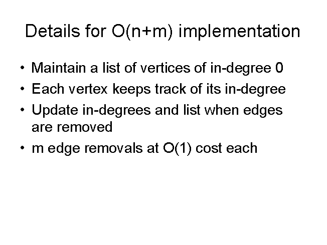
The discussion covers the points necessary for an efficient implementation of the algorithm.