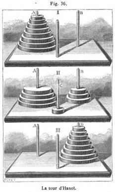
Figure 1. An early description of the problem “La Tour d’Hanoi” from the 1895 book by Edouard Lucas. Your program will determine an optimal policy for solving this puzzle, as well as compute utility values for each state of the puzzle.
CSE 415: Introduction to Artificial Intelligence
The University of Washington, Seattle, Spring 2021
Due: Friday, May. 14 via Gradescope at 11:59 PM.
Early Bird Bonus Deadline: Tuesday, May. 11 11:59 PM.
| Files you’ll edit: | |
solver_utils.py
|
Utilities for various reinforcement learning algorithms |
| Files you should read but NOT edit: | |
solvers.py
|
Reinforcement learning solvers for MDPs |
toh_mdp.py
|
Definitions for the TOH-world MDP |
| Files you will not edit: | |
autograder.py
|
Assignment autograder |
gui.py
|
Graphical User Interface for the TOH-world MDP |
test_cases
|
Test cases directory to support the autograder |
This assignment not only offers an opportunity to implement the Value Iteration algorithm, but also an opportunity to see how reinforcement learning techniques can be applied to problem solving of the sort we studied earlier with state-space search.
While due Friday, May. 14, the assignment has an early-bird option, in which you can turn in Part 1 by Tuesday, May. 11, for 5 points of extra credit.
The interactions between a problem-solving agent and its problem-domain environment are modeled probabilistically using the technique of Markov Decision Processes. Within this framework, the assignment focuses on two approaches to having the agent maximize its expected utility: (A) by a form of planning, in which we assume that the parameters of the MDP (especially the transition model \(T\) and the reward function \(R\)) are known, which takes the form of Value Iteration, and (B) by an important form of reinforcement learning, called Q-learning, in which we assume that the agent does not know the MDP parameters.
The particular MDPs we are working with in this assignment are variations of a “TOH World”, meaning Towers-of-Hanoi World. We can think of an agent as trying to solve a TOH puzzle instance by wandering around in the state space that corresponds to that puzzle instance. If it solves the puzzle, it will get a big reward. Otherwise, it might get nothing, or perhaps a negative reward for wasting time. In Part 1, the agent is allowed to know the transition model and reward function. In Part 2, the agent is not given that information, but has to learn it by exploring and seeing what states it can get to and how good they seem to be based on what rewards it can get and where states seem to lead to.
Download and unzip the starter code. Make sure you are using Python 3.9 which includes the Tkinter user-interface. Note that a specific dependency in Python 3.9 is not available on Windows so if Windows users see the error No module named 'tzdata', you can resolve it by running pip install tzdata.
In a command line, run
python gui.pyThis will start up a graphical user interface and can help you debug. You can see that some menus are provided. Some menu choices are handled by the starter code, such as setting some parameters of the MDP. However, you will need to implement the code to actually run the Value Iteration and the Q-Learning and some menu buttons will not work correctly until you implement the corresponding functions.
Figure 1. An early description of the problem “La Tour d’Hanoi” from the 1895 book by Edouard Lucas. Your program will determine an optimal policy for solving this puzzle, as well as compute utility values for each state of the puzzle.
The first thing you will probably notice is that our code, for the most part that you will be interacting with, are annotated with types. Python is a flexible language that’s great for prototyping small programs, and part of the flexibility comes from its nature as a dynamically typed language. In other words, all the type checking, if they exist at all, happens during runtime. This however has caused a lot of headaches for the past assignments since it is hard to know what kind of arguments a specific function is expecting, and therefore many students had a hard time tracking down the error. So for this assignment we type annotated our starter code to help you determine what’s an appropriate input to a function. Furthermore, if you use an IDE with strong support for static inference such as PyCharm, you’ll see an error if your code doesn’t type check. If you wish to read a quick introduction on Type Annotation, this document is a good place to start. If you wish you type check your code, you can consider the Python Software Foundation funded Python Type Checking program, mypy. You can install mypy with pip install mypy and type check your solution file with
mypy solver_utils.pyNote that mypy will throw a lot of errors if you haven’t completed all the questions. You may want to add some temporary values to suppress these errors before you actually implement those functions.
With a handful of exceptions, our entire starter code are compliant with the official Python style guide PEP 8 and an industrial extension Google Python Style Guide. We encourage you to follow the same tradition. Again, if you use PyCharm, PEP 8 violations will be pointed out to you.
The included autograder has a number of options. You can view it by
python autograder.py --helpSome commonly used flags are: --no-graphics, which disables displaying the GUI, -q which grades only one question, and -p, which grades a particular part.
Part 1 is mainly concerned with value iteration. Now would be a good time to review the Bellman equations.
You can test your Part 1 implementations with
python autograder.py -p p1In solver_utils.py, complete the function that computes one step of value iteration:
def value_iteration(
        mdp: tm.TohMdp, v_table: tm.VTable
) -> Tuple[tm.VTable, tm.QTable, float]:
    """..."""
Before you write any code, it would be a good idea to take a look at the toh_mdp.py file, which defines all the components of TOH world MDP. In particular, TohState, Operator, TohAction, and most importantly, TohMdp are the classes you will be interacting the most, and you should familiarise yourself with the way these objects interact with each other. When in doubt of the details of any functionality, the best way is to consult the documentation (provided as comments in the code) and the implementation itself.
Make sure you also read the documentation in the code to avoid some common pitfalls.
You can test your implementation with
python autograder.py -q q1The autograder will display your value iteration process for a sample TOH MDP. You might notice that the autograder logs lots of additional info. You can suppress this by setting LOGLEVEL from INFO to WARNING in your shell, i.e.,
LOGLEVEL=WARNING python autograder.py -q q1Note: Our reference solution takes 12 lines.
In solver_utils.py, complete the function that extracts the policy from the value table:
You can test your implementation with
python autograder.py -q q2The autograder will display your value iteration process for a sample TOH MDP as well as the policy during each iteration. You can observe how the policy changes as the values change. Finally, the autograder will simulate an agent’s movement using your learned policy. If your implementation is correct, your agent mostly follows the optimal trajectory. You can view the optimal path by selecting “MDP Rewards” -> “Show golden path (optimal solution)”.
Note: Our reference solution takes 2 lines.
You can test your Part 1 implementations with
python autograder.py -p p2Q learning performs an update on the Q-values table upon observing a transition, which in this case is represented as a \((S, A, R, S')\) tuple.
Implement the q_update function, which updates the q_table based on the observed transition, with the specified learning rate alpha:
def q_update(
        mdp: tm.TohMdp, q_table: tm.QTable,
        transition: Tuple[tm.TohState, tm.TohAction, float, tm.TohState],
        alpha: float) -> None:
You can test your implementation with
python autograder.py -q q3Note: Our reference solution takes 5 lines.
Q learning only works with the Q-value table, but sometimes it is useful to know the (estimated) value for a certain state. Implement the extract_v_table function, which computes a value table from the Q-value table:
You can test your implementation with
python autograder.py -q q4Note: Our reference solution takes 2 lines.
At the core of on-policy Q learning is the exploration strategy, and \(\epsilon\)-greedy is a commonly used baseline method. In this assignment, your agent is assumed to perform on-policy learning, i.e., the agent actively participates (chooses the next action) when acting and learning, instead of passively learn by observing a sequence of transitions. Implement the choose_next_action below.
def choose_next_action(
        mdp: tm.TohMdp, state: tm.TohState, epsilon: float, q_table: tm.QTable,
        epsilon_greedy: Callable[[List[tm.TohAction], float], tm.TohAction]
) -> tm.TohAction:
Make sure you use the supplied epsilon_greedy function to sample the action. You should not need to use the random module. That is handled for you in the QLearningSolver.epsilon_greedy function in solvers.py. Make sure you read its code.
You can test your implementation with
python autograder.py -q q5Note that this time the autograder will do a sanity check of your implementation first, and then use your exploration strategy to run for 10,000 Q learning steps with \(\epsilon=0.2\). You will receive full credit if after 10,000 Q updates, your agent is able to learn the optimal policy on the solution path (it’s ok if the policy for other states are suboptimal).
Note: Our reference solution takes 4 lines.
If you use a constant \(\epsilon\), you model will waste time exploring unnecessary states as time approaches infinity. A common way to mitigate this is to use a function for \(\epsilon\) that depends on the time step ( see the slide on GLIE: Greedy in the Limit with Infinite Exploration on this lecture note). Implement the custom_epsilon to design your function of \(\epsilon\):
You can test your implementation with
python autograder.py -q q6Same as Q5, the autograder is going to use your custom \(\epsilon\) function to perform Q learning, and you will receive full credit if after 10,000 Q updates, your agent is able to learn the optimal policy on the solution path (it’s ok if the policy for other states are suboptimal).
Note: Our reference solution takes 1 line.
Submit you solver_utils.py file to Gradescope. You can run the entire test suite with
python autograder.pyMay. 8, 4:28am: The number of Q updates in Q5 and Q6 are updated to 10,000 from 5,000. The default \(\epsilon\) value is set to 0.2 so that the autograder is more lenient. The starter code file is updated to reflect this change.
May. 8, 1:23pm: Python 3.9 is now required.
May. 8, 5:45pm: Added number of lines of code of our reference solution, so you don’t overthink too much.