Part 1 due: at 11pm on Thursday, July 26.
Part 2 due: at 11pm on Thursday, August 2.
Submit via
Catalyst
CollectIt (a.k.a. Dropbox).
In this assignment, you will try to detect fraud in a dataset, in two different ways:
This assignment will also give you practice with the basics of statistical testing.
To get started, download and extract the homework6.zip file.
You will write all your answers in a new file, fraud_detection.py, that you will create. In some cases, your answers will be Python code. In other cases, your answers will be textual, in which case you should write them as comments. For every problem, make sure that the code that answers it
Different parts of this assignment require similar, but not exactly identical, work. When you notice such repetition, you should refactor and generalize your code. That is, rather than writing two similar routines, you should write one routine that takes the place of both.
Part of your grade will depend on how little redundancy remains in the code you turn in.
Important: Leave yourself some time to go back and refactor your code before you turn it in.
In this part of the assignment, you will look for fraud in election returns from the disputed 2009 Iranian presidential election. You will examine the least significant digits of the vote totals — the ones place and the tens place.
The ones place and the tens place don't affect who wins. They are essentially random noise, in the sense that in any real election, each value is equally likely. Another way to say this is that we expect the the ones and tens digits to be uniformly distributed — that is, 10% of the digits should be "0", 10% should be "1", and so forth. If these digits are not uniformly distributed, then maybe the numbers were made up by a person rather than collected from ballot boxes. (People tend to be poor at making up random numbers.)
There were four candidates in the election: Ahmadinejad, Rezai, Karrubi, and Mousavi. File election-iran-2009.csv contains data, reported by the Iranian government, for each of the 30 provinces. Thus, there are 120 numbers we care about in the file. Write code to place these numbers in a single list.
Hint: Use csv.DictReader. You will also have to remove double-quotes and commas from the data, and convert them to numbers.
Write a function ones_digit that returns the last digit of a number, and a function tens_digit that returns the next-to-last digit of a number.
Write a function ones_digit_histogram that takes as input a list of numbers and produces as output a list of 10 numbers. Each element of the result indicates the frequency with which that digit appeared in the ones place in the input. Here is an example call and result:
>>> ones_digit_histogram([0, 1, 1, 2, 3, 5, 8, 13, 21, 34, 55, 89, 144, 233, 377, 610, 987, 1597, 2584, 4181, 6765])
[0.09523809523809523, 0.19047619047619047, 0.047619047619047616, 0.14285714285714285, 0.14285714285714285, 0.14285714285714285, 0, 0.14285714285714285, 0.047619047619047616, 0.047619047619047616]
Write a function ones_and_tens_digit_histogram that takes as input a list of numbers and produces as output a list of 10 numbers. Each element of the result indicates the frequency with which that digit appeared in the ones place or the tens place in the input. Here is an example call and result:
>>> ones_and_tens_digit_histogram([0, 1, 1, 2, 3, 5, 8, 13, 21, 34, 55, 89, 144, 233, 377, 610, 987, 1597, 2584, 4181, 6765])
[0.21428571428571427, 0.14285714285714285, 0.047619047619047616, 0.11904761904761904, 0.09523809523809523, 0.09523809523809523, 0.023809523809523808, 0.09523809523809523, 0.11904761904761904, 0.047619047619047616]
Hint: in a number that is less than 10, such as 3, the tens place is implicitly zero. Your code should treat it as zero.
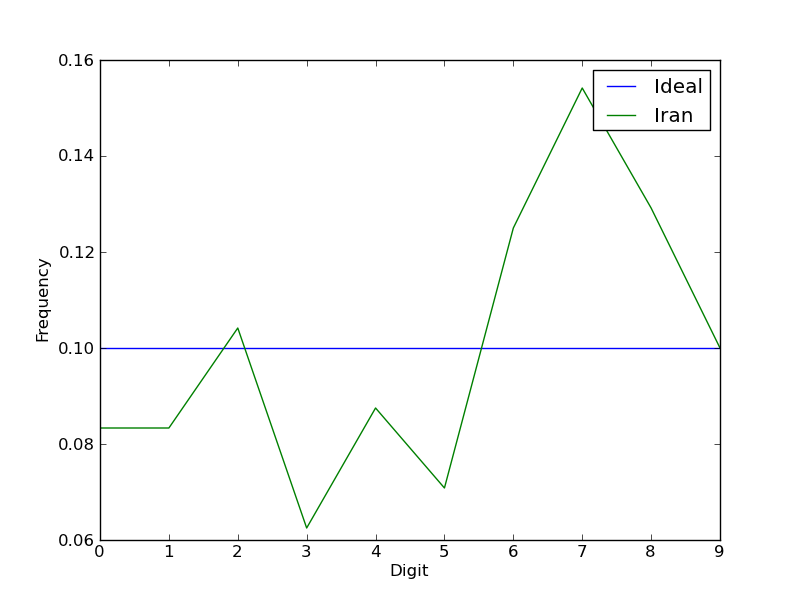
Write a function that graphs the frequencies of the ones and tens digits, for the Iranian election data. The result should look just like this one. Don't forget the x- and y-axis labels and the legend. Use pyplot.plot for the line itself.

Save your plot to a file named iran-digits.pdf. Hint: use pyplot.savefig.
The data are rather different from the expected flat line at y=.1. Are these data different enough that we can conclude that the numbers are probably fake? You can't tell just by looking at the graphs we have created so far. We will show more principled, statistical ways of making this determination.
With a small sample, the vagaries of random choice might lead to results that seem different than expected. As an example, suppose that you plotted a histogram of 20 randomly-chosen digits (10 random numbers, 2 digits per number):
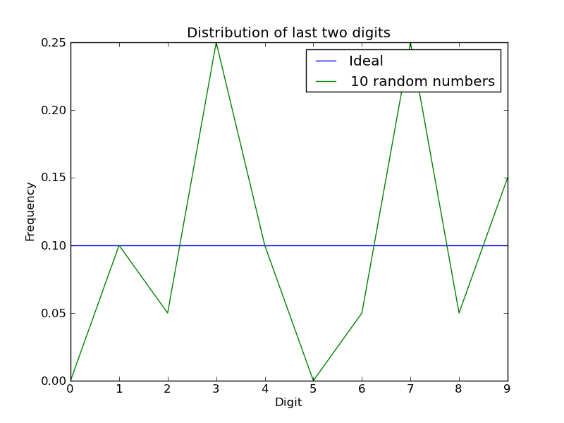
That looks much worse than the Iran data, even though it is genuinely random! Just because your observations do not seem to fit a hypothesis does not mean the hypothesis is false — maybe you have not yet examined enough data to see the trend.
Write a function random_two_digits that takes a number and returns a list of the given length, where each value is an integer randomly chosen in the range [0,99]. Hint: use random.randint.
Write a function that creates a graph. The graph should look like the figure above (note the title, legend, and x- and y-axis labels), but it should have 5 plots, for 10, 50, 100, 1000, and 10000 random numbers. Naturally, random variation will make your graph look different than this one (and it's likely to be different from run to run of your program).
Save your plot to the filename random-digits.pdf.
Observing your plot demonstrates that the more datapoints there are, the closer the result is to the ideal histogram. We must take the sample size into account when deciding whether a given sample is suspicious.
You can visually see that some graphs are closer to the ideal than others. But, we would like a way to determine that computationally.
We would like a way to determine how similar two graphs are — and more specifically, we would like to determine whether the difference between graphs A and B is larger or smaller than the difference between graphs C and D. For this, we will define a distance metric. Given two graphs, it returns a number — a distance — that is 0 if the two graphs are identical, and is larger the more different two graphs are.
One common measure for the difference/distance between two datasets is the mean squared error. For each corresponding datapoint, compute the difference/distance between the two points, then square it. The overall distance measure is the sum of the squares. (The use of squares means that one really big difference among corresponding datapoints is more important than several small differences.)
For example, suppose that you had the data that appears in the following table and plot:
| x | f(x) | g(x) | h(x) |
|---|---|---|---|
| 1 | 1 | 2 | 6 |
| 2 | 4 | 3 | 5 |
| 3 | 9 | 4 | 4 |
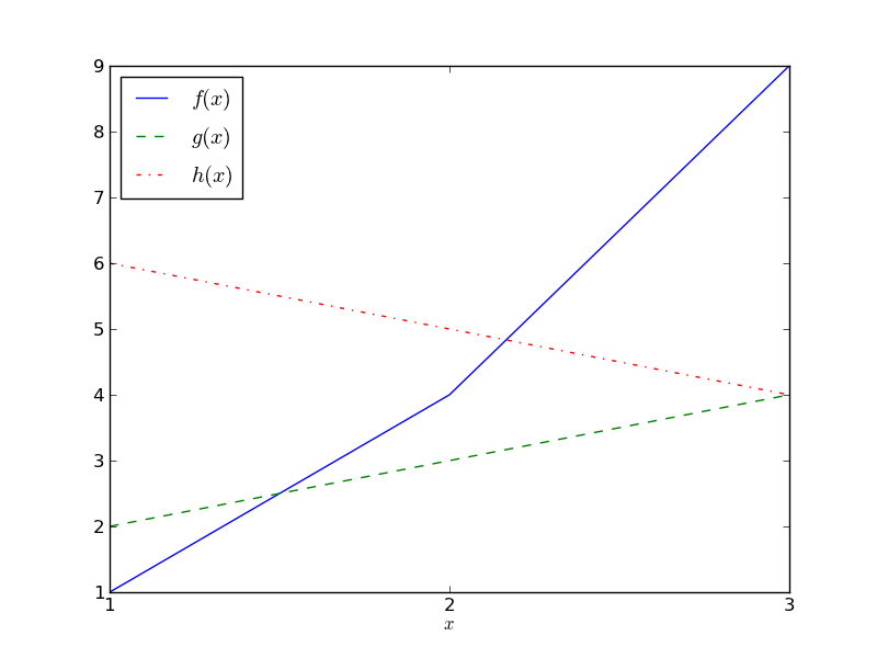
The MSE difference between f and g is
(1-2)2 +
(4-3)2 +
(9-4)2 = 27.
The MSE difference between f and h is
(1-6)2 +
(4-5)2 +
(9-4)2 = 51.
The MSE difference between g and h is
(2-6)2 +
(3-5)2 +
(4-4)2 = 20.
The absolute values of the MSE are not interesting; it's only comparisons
between them that are. These numbers show that
g and h are the most similar, and
f and h are the most different.
Write a function mse that, given two lists of numbers, computes the mean squared error between the lists.
Imagine conducting infinitely many elections in the same way as the 2009 Iranian election (including with or without fraud). That would produce infinitely much data. The 120 datapoints that you have is a small sample of that very large dataset. We don't know what that large dataset is, but we want to answer a question about it: does that dataset have uniformly-distributed ones and tens digits? If, just from looking at our small sample, we can determine that the large unknown dataset does not have uniformly-distributed ones and tens digits, then we can conclude that the observed sample is fraudulent (it came from some other source, such as some bureaucrat's imagination).
One sample can't conclusively prove anything about the underlying distribution. For example, there is a very small possibility that, by pure coincidence, a fair election might produce 120 numbers that all end with "11". If we saw a sample whose ones-and-tens-digit histogram is all 1, we would be quite sure, but not 100% sure, that the data is fraudulent.
Our methodology is as follows: We take as an assumption that the observed sample (the Iranian election data) is not fraudulent — we call this the "null hypothesis". Our question is whether we can, with high likelihood, reject that assumption. Our specific question is, "What is the likelihood that the Iranian election data is a sample of a large unknown dataset whose least significant digits are uniformly distributed?"
Augment your program to compute and print the mean squared error between the uniform distribution and the Iranian election results histogram (for the ones and tens digits). You should obtain the result 0.00739583333333, or approximately 0.007.
This number on its own does not mean anything — we don't know whether it is unusually low, or unusually high, or about average. To find out, we need to compare it to similarly-sized sets.
Compute the MSE distance for 10000 sets of random numbers, where each set is the same size as the Iranian election data. Then, determine where the value 0.007 appears in that list. In other words, determine how many of the random MSEs are larger than the Iran MSE, and how many of the random MSEs are smaller than the literature MSE.
Put your answer in a comment in your source file, near the code that computes it.
Here are some possibilities for the outcome of the previous question:
By convention, when an event is more than 5% likely, we state that it does not provide any statistically significant evidence against the null hypothesis. This means that, by convention, when an event is reported as statistically significant, there is a 1/20 or less chance that it is just a fluke caused by unlucky (or lucky) random choices.
(Actually, this fit is remarkably close to the theoretical ideal — much closer than one would typically expect a randomly-chosen sample of that size to be. But, it would come up once in a while, and maybe this is one of those times. Or maybe the data were fudged to look really, really natural — too natural, suspiciously natural. In any event, this result does not give grounds for accusing the election authorities of fraud, given what we were measuring.)
Suppose that you are only testing genuine, non-fraudulent elections. Then, 1 time in 20, the above procedure will cause you to cry foul and make an incorrect accusation of fraud. This is called a false alarm or false positive or Type I error. It is an inevitable risk of statistics. If you run enough different statistical tests, then by pure chance some of them will (seem to) yield a result. You can reduce the chance of such an error by reducing the 5% threshold discussed above. Doing so makes your test less sensitive: your test will more often suffer a failed alarm or false negative or Type II error, where there really was an effect but you missed it.
There are better, closed-form formulas for computing statistical confidence. But, we do not want to burden you with sophisticated math that you may not understand. More importantly, this idea of performing many trials, and seeing how likely or unlikely the real data are, is at the heart of all statistics, and it is more important than understanding a set of formulas.
If you are interested, Wikipedia has more on hypothesis testing. Reading this is optional, however.
Interpret your results. State whether the data suggest that the Iran election results were tampered with before being reported to the press. Briefly justify your answer.
We have provided you with another dataset, from the 2008 US presidential election. It appears in file election-us-2008.csv, and is taken from Wikipedia. Consider the null hypothesis that it was generated according to a uniform distribution of ones and tens digits. State whether you can reject that hypothesis, and with what confidence.
As extra credit, also evaluate data from the recent 2012 Egpytian presidential election. You can find the data at Wikipedia.
Submit your work. Don't forget the collaboration and reflection sections, in a file named answers.txt.
For part 2 of the current homework, please use the *same* fraud_detection.py file that you used in part 1 -- augment it with new code. You will submit that same file again.
Suppose that you measure some naturally-occurring phenomenon, such as the land area of cities or lakes, or the price of stocks on the stock market. You can plot a histogram of of the first digits of your measurements, showing how frequent each first digit (1-9) is.
Your measurements were made in some arbitrary units, such as square miles or dollars. What if you made the measurements in some other units, such as acres or euros? You would not expect the shape of the histogram to differ just because you changed the units of measurement, because the units are arbitrary and unrelated to the underlying phenomenon. If the shape of the histogram did change, that could indicate that the data were fraudulent. This approach has been used to detect fraud, especially in accounting and economics but also in science.
Data are called scale invariant if measuring them in any scale (say, meters vs. feet vs. inches) yields similar results, such as the same histogram of first digits. Many natural processes produce scale-invariant data. Benford's Law states the remarkable fact there is only one possible histogram that results from all of these processes! Let P(d) be the probability of the given digit being the first one in a measurement. Then, the probabilities of the digits are shown in this table (from Wikipedia).
| d | P(d) | Relative size of P(d) |
|---|---|---|
| 1 | 30.1% |
|
| 2 | 17.6% |
|
| 3 | 12.5% |
|
| 4 | 9.7% |
|
| 5 | 7.9% |
|
| 6 | 6.7% |
|
| 7 | 5.8% |
|
| 8 | 5.1% |
|
| 9 | 4.6% |
|
Benford's law only holds when the data has no natural limit nor cutoff. For example, it would not hold for grades in a class (which are in the range 0% to 100% or 0.0 to 4.0) nor for people's height in centimeters (where almost every value would start with 1 or 2). If you are interested, Wikipedia has more information about Benford's law. Reading the Wikipedia article is optional, however.
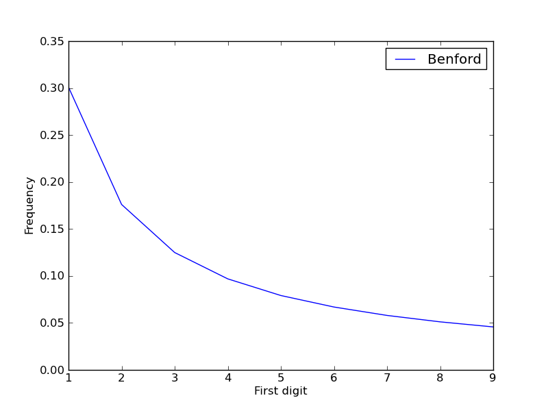
The histogram of first digit values for a distribution obeying Benford's Law can be computed as P(d) = log10(1 + 1/d).
Using that formula, create a plot that looks just like this one. Don't forget the x- and y-axis labels and the legend. Use pyplot.plot for the line itself.
In this part of the problem, you will create artificial data that obeys Benford's Law.
Here is one way to generate datapoints that obey Benford's Law:
Generate 1000 datapoints using the above technique.
On your graph from Problem 9, draw another line, labeled "1000 samples", that plots the frequency of first digits among your 1000 datapoints. Don't use the pyplot.hist routine — just use pyplot.plot, as you did above.
Hint: You will find it helpful to write helper functions, such as first_digit and first_digit_histogram, much as you did in Part 1.
In this problem, you will see that the scale-invariance property holds.
Add another line to your plot from Problem 10. It will be like the line you just added, but each datapoint is computed as π × er. For the label in the legend, use "1000 samples, scaled by $\pi$". (The funny "$\pi$" will show up as a nicely-formatted π in the graph.)
Save your plot to the filename scale-invariance.pdf. You will turn it in. It should have 3 functions graphed on it.
Compare your two plots. There are some differences due to random choices, but overall it demonstrates the scale-independence of the distribution you just created. It also demonstrates the scale-independence of the Benford distribution, since it is so similar to the one you just created. (It is possible to demonstrate the scale-independence of Benford's Law mathematically as well. You are welcome to try doing this, but it is not required.)
We wish to know whether the population of cities in the United States follows Benford's Law.
Your directory contains a file SUB-EST2009_ALL.csv. with United States census data. The file is in "comma-separated values" format. Python's csv.reader can parse this format.
On a new graph, plot the histogram of first digits that obey Benford's Law, just as you did in Problem 9. Also plot the data from the "POPCENSUS_2000" column of the file, and give it the label "US (all)".
Your graph now has two curves plotted on it. From the similarity of the two curves, you can see that the population of U.S. cities obeys Benford's Law.
The file literature-population.txt contains the populations of various places that appear in literature and pop culture. We would like to know whether these populations are characteristic of real population counts, in the sense of obeying Benford's Law equally well.
Plot the data from the file literature-population.txt on the same graph from Problem 12. Notice that the data are similar to, but not exactly the same as, the the real dataset and the perfect Benford's-Law histogram.
Are these data far enough from obeying Benford's Law that we can conclude that the numbers are fake? Or are they close enough to obeying Benford's Law that they are statistically indistinguishable from real data? You can't tell just by looking at the graphs we have created so far. We will show more principled, statistical ways of making this determination.
The larger a sample is, the closer it is to the ideal distribution. With smaller samples, the vagaries of random choice might lead to results that seem different than random. As an extreme example, suppose that you plotted a histogram of just the first 10 cities in the SUB-EST2009_ALL.csv file. (You don't have to do this for the assignment.) It would look like this:
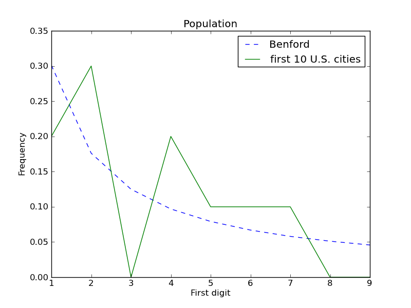
This graph is rather different from the Benford's-Law histogram, but that does not necessarily mean that city populations do not obey Benford's Law — maybe you have not yet examined enough data to see the trend.
Revisit your graph that plotted randomly-generated data, from Problem 10. Currently, you have a plot containing Benford's Distribution and 1000 randomly-selected points. Augment your graph, adding plots for 10, 50, 100, and 10000 randomly-selected points. Your final graph will plot 6 curves.
Save your plot to the filename benford-samples.pdf.
Notice that the larger the sample size, the closer the distribution of first digits approaches the theoretically perfect distribution. This demonstrates that the more datapoints there are, the closer it is to the true distribution.
A distribution is a process that can generate arbitrarily many datapoints. A distribution obeys Benford's Law if, after choosing infinitely many points, the frequency of first digits is exactly P(d) = log10(1 + 1/d).
A sample is a finite set of measurements. We wish to know whether it is possible that these measurements were chosen from some distribution that obeys Benford's Law.
The literature place populations is a small sample — just a few dozen datapoints. If, just from looking at our small sample, we can determine that the unknown distribution they came from does not obey Benford's Law, then we can conclude that the observed sample is not genuine. We can conclude that because place populations from the United States and elsewhere in the real world do obey Benford's Law.
One sample can't conclusively prove anything about the underlying distribution. For example, there is a very small possibility that, by pure coincidence, we might randomly choose 100 numbers that all start with the digit 1. If we saw a sample of 100 datapoints whose first-digit histogram is all 1, we would be quite sure, but not 100% sure, that the underlying distribution does not obey Benford's Law. We might say that we are more than 99.9% sure that the data is fraudulent.
So, our question is, "What is the likelihood that the literature place populations are a sample of an unknown distribution that does not obey Benford's Law?" In other words, if we had to bet on whether the literature place populations are fraudulent, what odds would we give? We will determine an answer to this question.
We take as an assumption that the observed sample (the literature place populations) are not fraudulent — we call this the "null hypothesis". Our question is whether we can, with high likelihood, reject that assumption. Rejecting the assumption means determining that the sample is fraudulent. By "fraudulent", here we mean that it was generated by some other process — such as human imagination — than the natural process that generates real population data.
Compute the mean squared error between Benford's distribution and the histogram of first digits of populations of literature places. You should obtain the result 0.00608941252081, or approximately 0.006.
This number on its own does not mean anything — we don't know whether it is unusually low, or unusually high, or about average. To find out, we need to compare it to similarly-sized sets.
Compute the MSE distance for 10000 sets of towns, where each set is randomly chosen to be of the same size as the list of literature places. Call this list the "US MSEs". Then, determine where the value 0.006 appears in that list. In other words, determine how many of the US MSEs are larger than the literature MSE, and how many of the US MSEs are smaller than the literature MSE.
Implementation tip: Suppose that you have a list of all the town populations in the United States. You can use the random.sample routine to randomly create a subset of a given size.
Interpret your results. Is there evidence that the literature place populations were artificially generated? Hint: you may wish to use a similar approach to that you used in Problem 9.
You are almost done!
Look over your work to find ways to eliminate repetition in it. Then, refactor your code to eliminate that repetition. This is important when you complete each part, but especially important when you complete part 2. When turning in part 2, you should refactor throughout the code, which will probably include more refactoring in part 1. You will find that there is some similar code within each part that does not need to be duplicated, and you will find that there are also similarities across the two parts. You may want to restructure some of your part 1 code to make it easier for you to reuse in part 2.
At the bottom of your answers.txt file, in the “Collaboration” part, state which students or other people (besides the course staff) helped you with the assignment, or that no one did.
At the bottom of your answers.txt file, in the “Reflection” part, state how many hours you spent on this assignment. Also state what you or the staff could have done to help you with the assignment.
Submit the following files via Catalyst CollectIt (a.k.a. Dropbox):